Week 6: Discussion Section

Source Materials

The following materials are modified from curriculum developed by Earth Lab and the Raster Analysis with terra book.

Many ways to plot a false color image

You can plot false color composites with ggplot2 too! Check out this tutorial.

In Lab #6, you explored various band combinations and plotted false color images with tm_rgb() from {tmap}. False color images allow you to visually highlight specific features in an image that may otherwise not be readily discernible. To add to your toolbelt, you will now be plotting false color images with plotRGB() from {terra}.

The plotRGB() function allows you to apply a stretch to normalize the colors in an image. You can either apply a linear stretch or histogram equalization. A linear stretch distributes the values across the entire histogram range defined by the max/min lower bounds of the original raster. A histogram equalization stretches dense parts of the histogram and condenses sparse parts.

But why would you want to normalize the colors in an image?

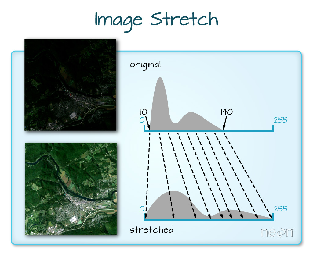
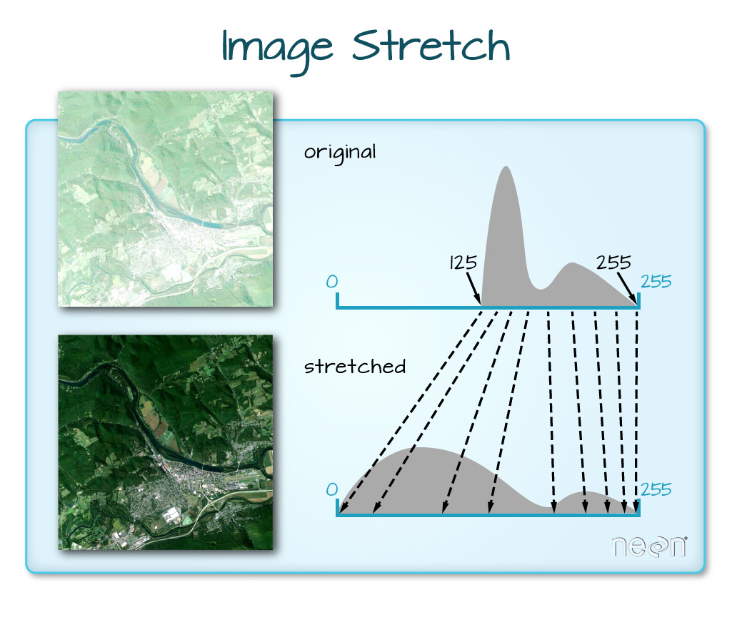
“When the range of pixel brightness values is closer to 0, a darker image is rendered by default. You can stretch the values to extend to the full 0-255 range of potential values to increase the visual contrast of the image. When the range of pixel brightness values is closer to 255, a lighter image is rendered by default. You can stretch the values to extend to the full 0-255 range of potential values to increase the visual contrast of the image.”

You are provided Landsat data for the site of the Cold Springs fire that occurred near Nederland, CO. The fire occurred from July 10-14, 2016 and the Landsat images are from June 5, 2016 (pre-fire) and August 8, 2016 (post-fire). The multispectral bands, wavelength range, and associated spatial resolution of the first 7 bands in the Landsat 8 sensor are listed below.

Band	Wavelength range (nanometers)	Spatial Resolution (m)	Spectral Width (nm)
Band 1 - Coastal aerosol	430 - 450	30	2.0
Band 2 - Blue	450 - 510	30	6.0
Band 3 - Green	530 - 590	30	6.0
Band 4 - Red	640 - 670	30	0.03
Band 5 - Near Infrared (NIR)	850 - 880	30	3.0
Band 6 - Short-Wave Infrared 1 (SWIR1)	1570 - 1650	30	8.0
Band 7 - Short-Wave Infrared 2 (SWIR2)	2110 - 2290	30	18

1. Get Started

• Create a version-controlled R Project
• Add (at least) a subfolder to your R project: data
• Create a Quarto document

Let’s load all necessary packages:

library(tidyverse)
library(sf)
library(terra)
library(tmap)
library(tmaptools)

Next, let’s download our data. Unzip and move this to your version-controlled R Project’s data folder.

# Set directory for folder
pre_fire_dir <- here::here("data", "LC80340322016189-SC20170128091153")

# Create a list of all images that have the extension .tif and contain the word band
pre_fire_bands <- list.files(pre_fire_dir,
                             pattern = glob2rx("*band*.tif$"),
                             full.names = TRUE)
# Create a raster stack
pre_fire_rast <- rast(pre_fire_bands)

# Read mask raster
pre_mask <- rast(here::here("data", "LC80340322016189-SC20170128091153", "LC80340322016189LGN00_cfmask_crop.tif"))

# Set directory for folder
post_fire_dir <- here::here("data", "LC80340322016205-SC20170127160728")

# Create a list of all images that have the extension .tif and contain the word band
post_fire_bands <- list.files(post_fire_dir,
                             pattern = glob2rx("*band*.tif$"),
                             full.names = TRUE)
# Create a raster stack
post_fire_rast <- rast(post_fire_bands)

# Read mask raster
post_mask <- rast(here::here("data", "LC80340322016189-SC20170128091153", "LC80340322016205LGN00_cfmask_crop.tif"))

And define the nbr_fun function to calculate the normalized burn ratio (NBR):

nbr_fun <- function(nir, swir2){
    (nir - swir2)/(nir + swir2)
}

2. Rename and mask the bands

Dealing with clouds and shadows

“Extreme cloud cover and shadows can make the data in those areas, un-usable given reflectance values are either washed out (too bright - as the clouds scatter all light back to the sensor) or are too dark (shadows which represent blocked or absorbed light)” (Earth Lab)

• Rename the bands of the pre_fire and post_fire rasters using names()

• Mask out clouds and shadows of the pre_mask and post_mask rasters (i.e., set mask > 0 to NA)

Solution

# Rename bands
bands <- c("Aerosol", "Blue", "Green", "Red", "NIR", "SWIR1", "SWIR2")
names(pre_fire_rast) <- bands
names(post_fire_rast) <- bands

# Set all cells with values greater than 0 to NA
pre_mask[pre_mask > 0] <- NA

# Subset raster based on mask
pre_fire_rast <- mask(pre_fire_rast, mask = pre_mask)

# View raster
plot(pre_fire_rast)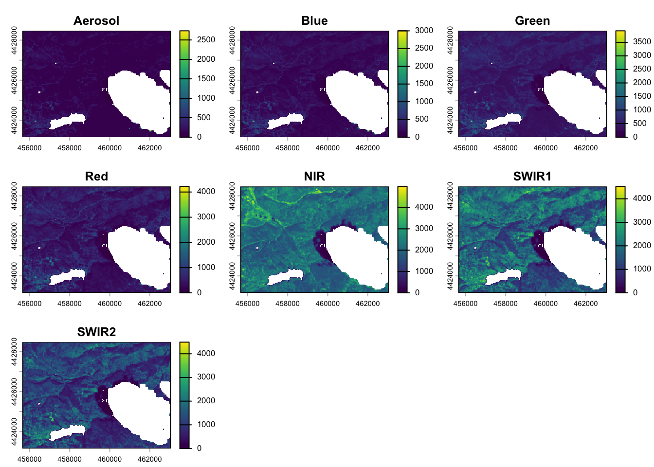

# Set all cells with values greater than 0 to NA
post_mask[post_mask > 0] <- NA

# Subset raster based on mask
post_fire_rast <- mask(post_fire_rast, mask = post_mask)

# View raster
plot(post_fire_rast)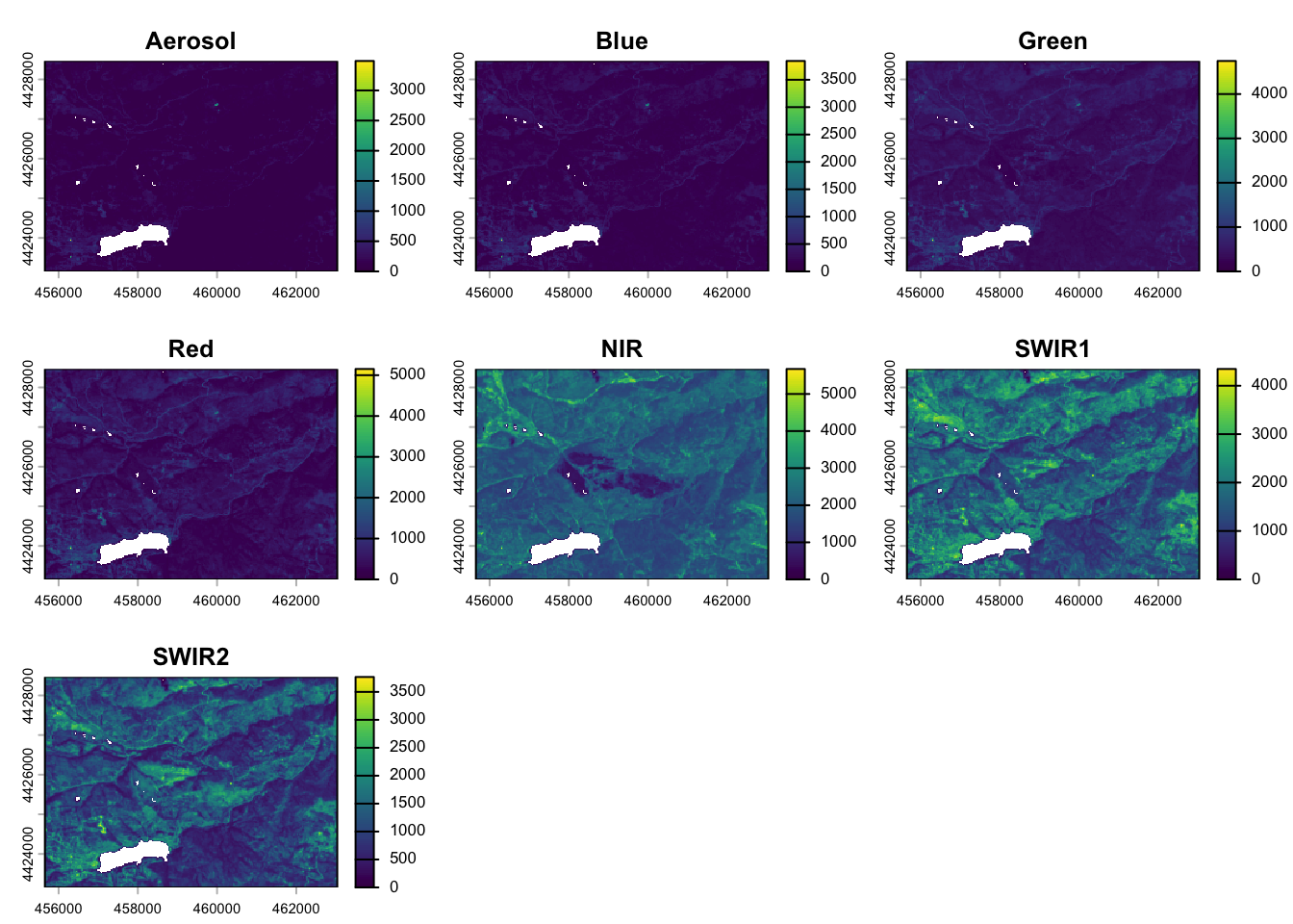

3. Plot true and false color composites

• Plot a true color composite using plotRGB()
  • Map the red band to the red channel, green to green, and blue to blue
  • Apply a linear stretch “lin” or histogram equalization “hist”

How to decide how to stretch a raster image?

To make an informed choice about whether to apply a linear stretch or histogram equalization, check the distribution of reflectance values of the bands in each raster:

# View histogram for each band
hist(pre_fire_rast,
     maxpixels = ncell(pre_fire_rast),
     col = "orange")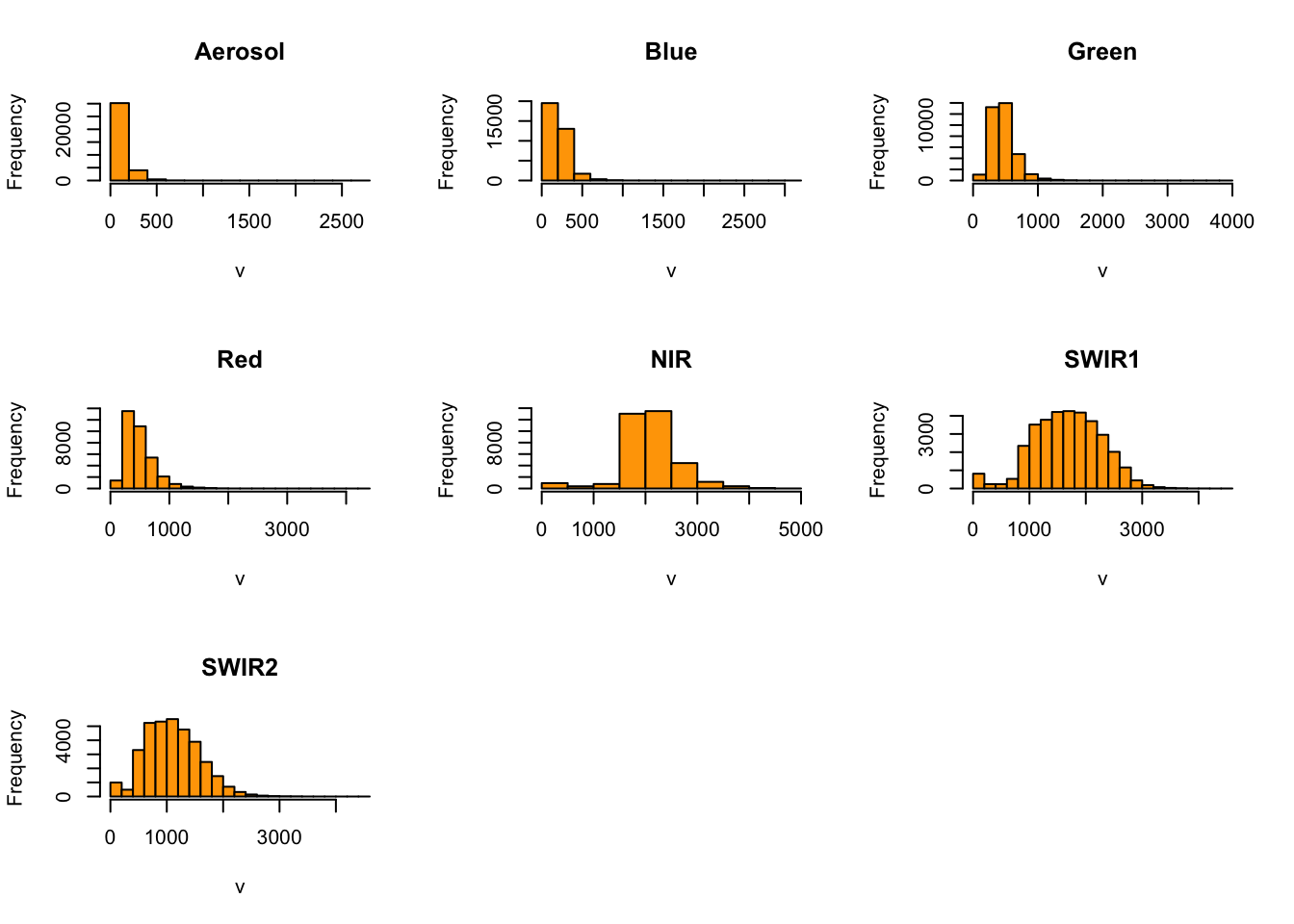

Solution

plotRGB(pre_fire_rast, r = 4, g = 3, b = 2, stretch = "lin", colNA = "black")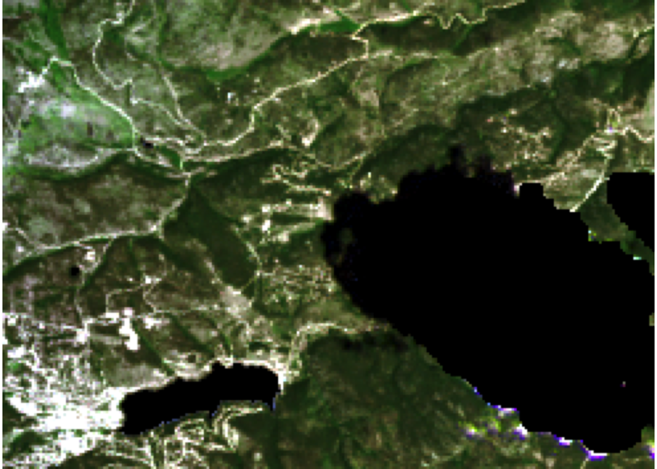

plotRGB(post_fire_rast, r = 4, g = 3, b = 2, stretch = "lin", colNA = "black")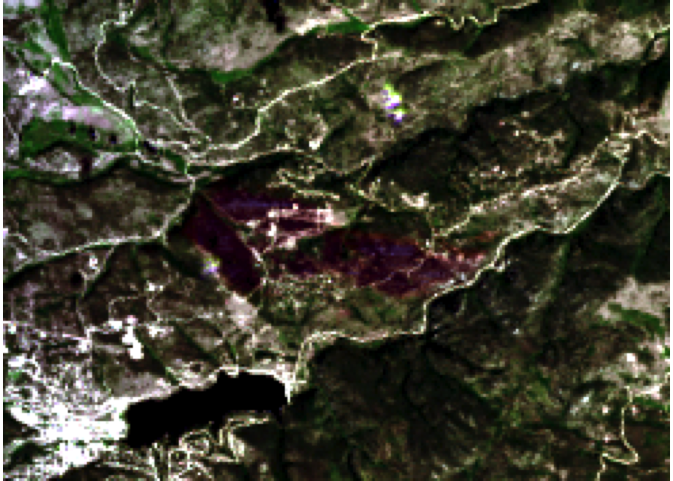

• Plot two false color composite using plotRGB()
  • Map the SWIR2 band to the red channel, NIR to green, and green to blue
  • Apply a linear stretch “lin” or histogram equalization “hist”

What is the SWIR, NIR, Red false color scheme?

“Combining SWIR, NIR, and Red bands highlights the presence of vegetation, clear-cut areas and bare soils, active fires, and smoke; in a false color image” (EOS Data Analytics)

Solution

plotRGB(pre_fire_rast, r = 7, g = 5, b = 3, stretch = "lin", colNA = "black")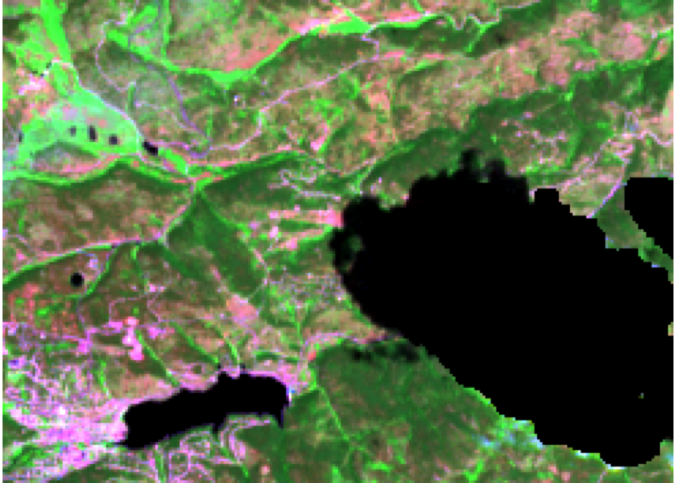

plotRGB(post_fire_rast, r = 7, g = 5, b = 3, stretch = "lin", colNA = "black")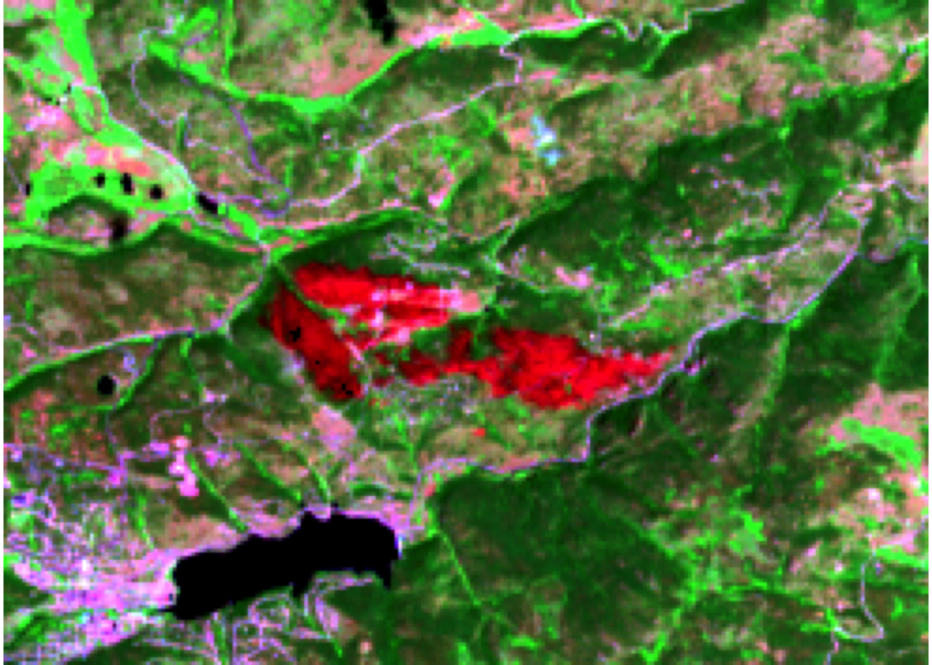

4. Calculate the normalized burn ratio (NBR)

• Calculate the normalized burn ratio (NBR)
  • Hint: Use lapp() like you previously did for NDVI and NDWI in Week 4

Solution

pre_nbr_rast <- terra::lapp(pre_fire_rast[[c(5, 7)]], fun = nbr_fun)

plot(pre_nbr_rast, main = "Cold Springs Pre-Fire NBR", colNA = "black")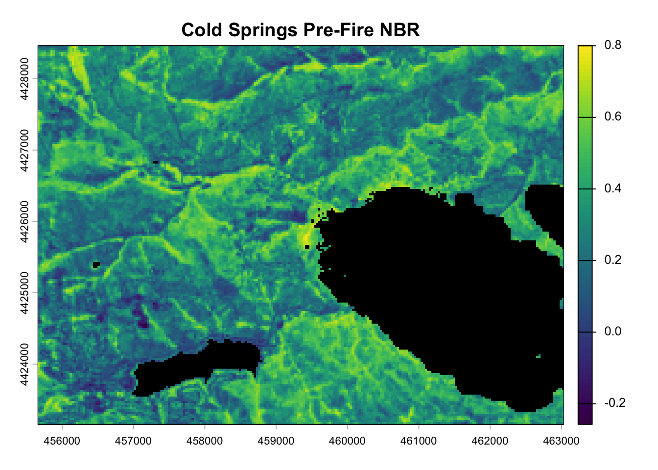

post_nbr_rast <- terra::lapp(post_fire_rast[[c(5, 7)]], fun = nbr_fun)

plot(post_nbr_rast, main = "Cold Springs Post-Fire NBR", colNA = "black")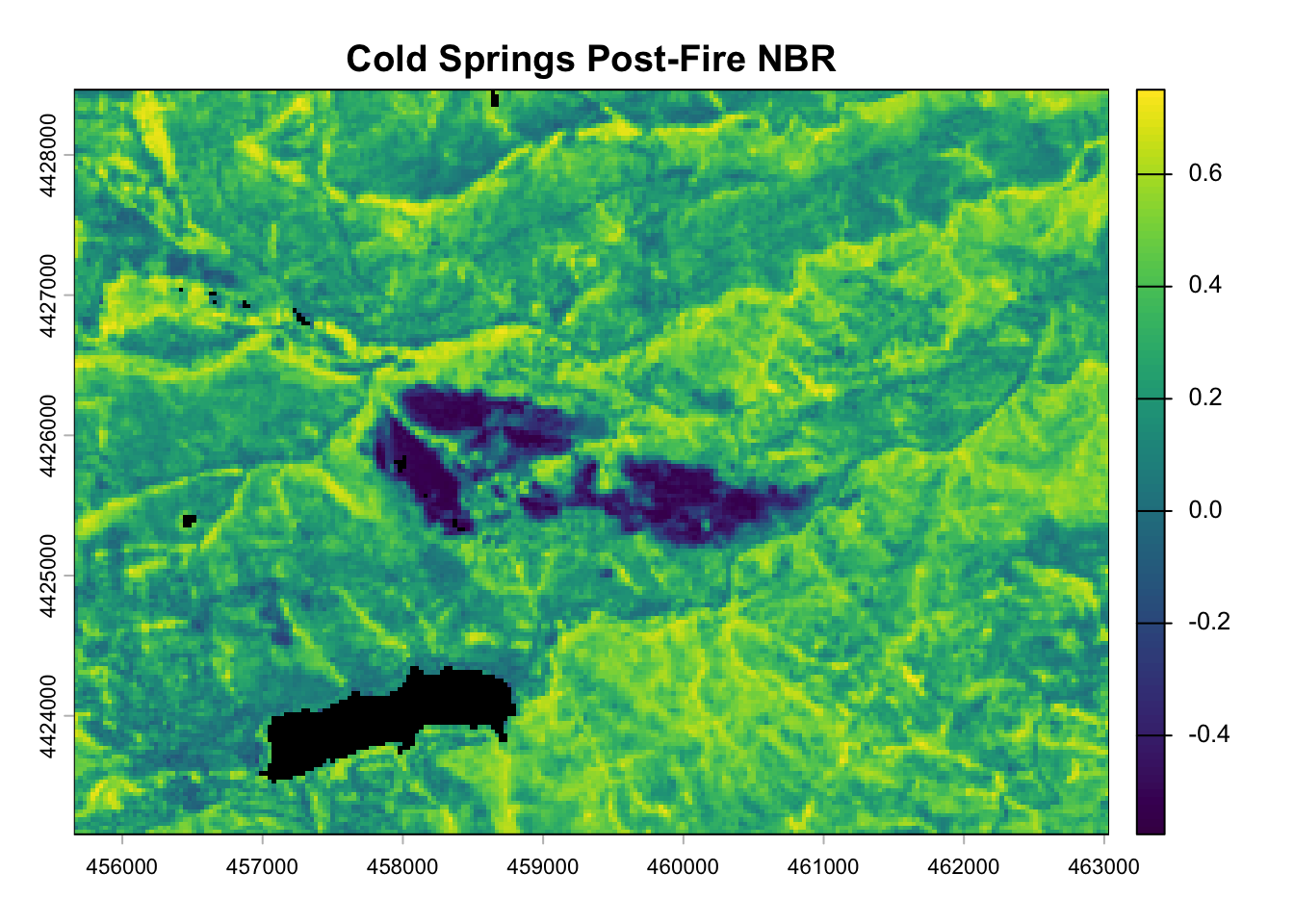

6. Calculate and plot difference NBR

• Find the difference NBR, where \(\text{d}NBR = \text{prefire}NBR- \text{postfire}NBR\)
• Plot the dnBR raster

Solution

diff_nbr <- pre_nbr_rast - post_nbr_rast

tm_shape(diff_nbr) +
  tm_raster(style = "equal", n = 6, 
            palette = get_brewer_pal("YlOrRd", n = 6, plot = FALSE),
            title = "Difference NBR (dNBR)", colorNA = "black") +
  tm_layout(legend.outside = TRUE)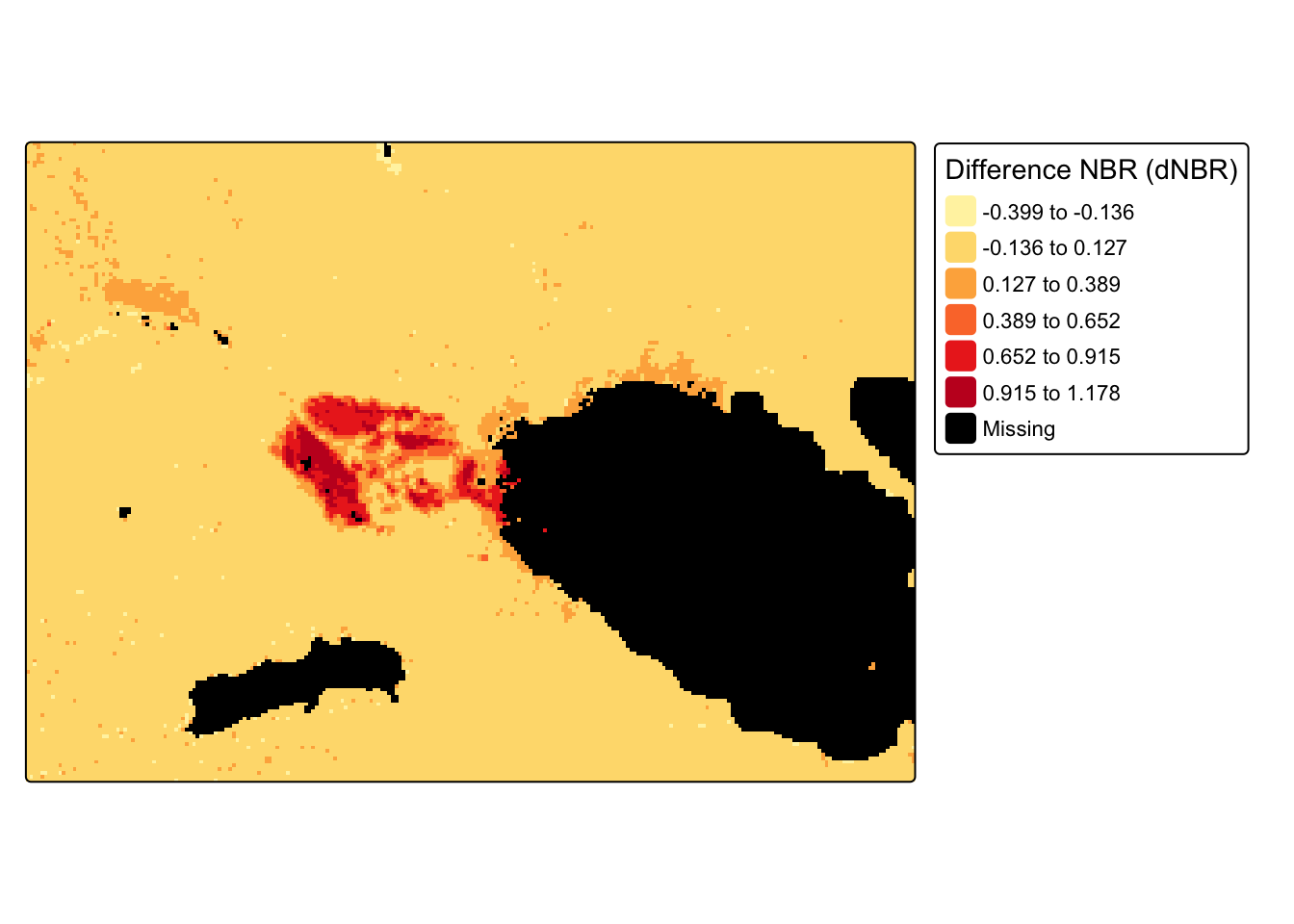

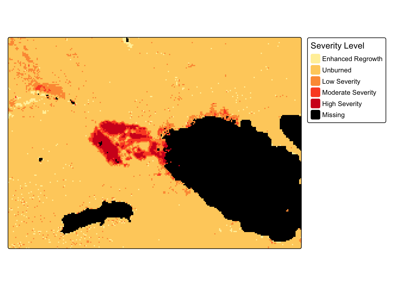
5. Bonus challenge: Classify severeity levels of burn

• Use classify() to assign the severity levels below:

Severity Level	dNBR Range
Enhanced Regrowth	< -.1
Unburned	-.1 to +.1
Low Severity	+.1 to +.27
Moderate Severity	+.27 to +.66
High Severity	> .66

Solution

# Set categories for severity levels
categories <- c("Enhanced Regrowth", "Unburned", "Low Severity", "Moderate Severity", "High Severity")

# Create reclassification matrix
rcl <- matrix(c(-Inf, -0.1, 1, # group 1 ranges for Enhanced Regrowth
                -0.1, 0.1, 2, # group 2 ranges for Unburned
                0.1, 0.27, 3, # group 3 ranges for Low Severity
                0.27, 0.66, 4, # group 4 ranges for Moderity Severity
                0.66, Inf, 5), # group 5 ranges for High Severity
                ncol = 3, byrow = TRUE)

# Use reclassification matrix to reclassify dNBR raster
reclassified <- classify(diff_nbr, rcl = rcl)

reclassified[is.nan(reclassified)] <- NA

tm_shape(reclassified) +
  tm_raster(style = "cat",
            labels = c(categories, "Missing"),
            palette = get_brewer_pal("YlOrRd", n = 5, plot = FALSE),
            title = "Severity Level", colorNA = "black")+
  tm_layout(legend.outside = TRUE)