Week 3: Lab

Artwork by Allison Horst

NoteSource Materials

The following materials are modified from Chapter 4 and Chapter 5 of Geocomputation with R by Robin Lovelace.

In this lab, we’ll explore the basics of spatial and geometry operations on vector data in R using the sf package. We’ll be working with data representing the heigh points of New Zealand.

Photo from Unsplash

Spatial data operations

Last week, we covered how the basics of the sf package. We saw that the magic of working with spatial data in the tidyverse means that we can leverage many of our favorite dplyr functions to manipulate the data attributes. So far, we’ve only worked with the data.frame component of sf objects. In this section, we’ll see how we can perform analogous operations using the geometry column.

1. Set Up

Let’s load all necessary packages:

library(sf)
library(tmap)
library(tidyverse)
library(spData)

2. Spatial subsetting (filtering)

When working with tabular data, we have frequently found it useful to subset the data.frame we are working with based on some condition using dplyr::filter().

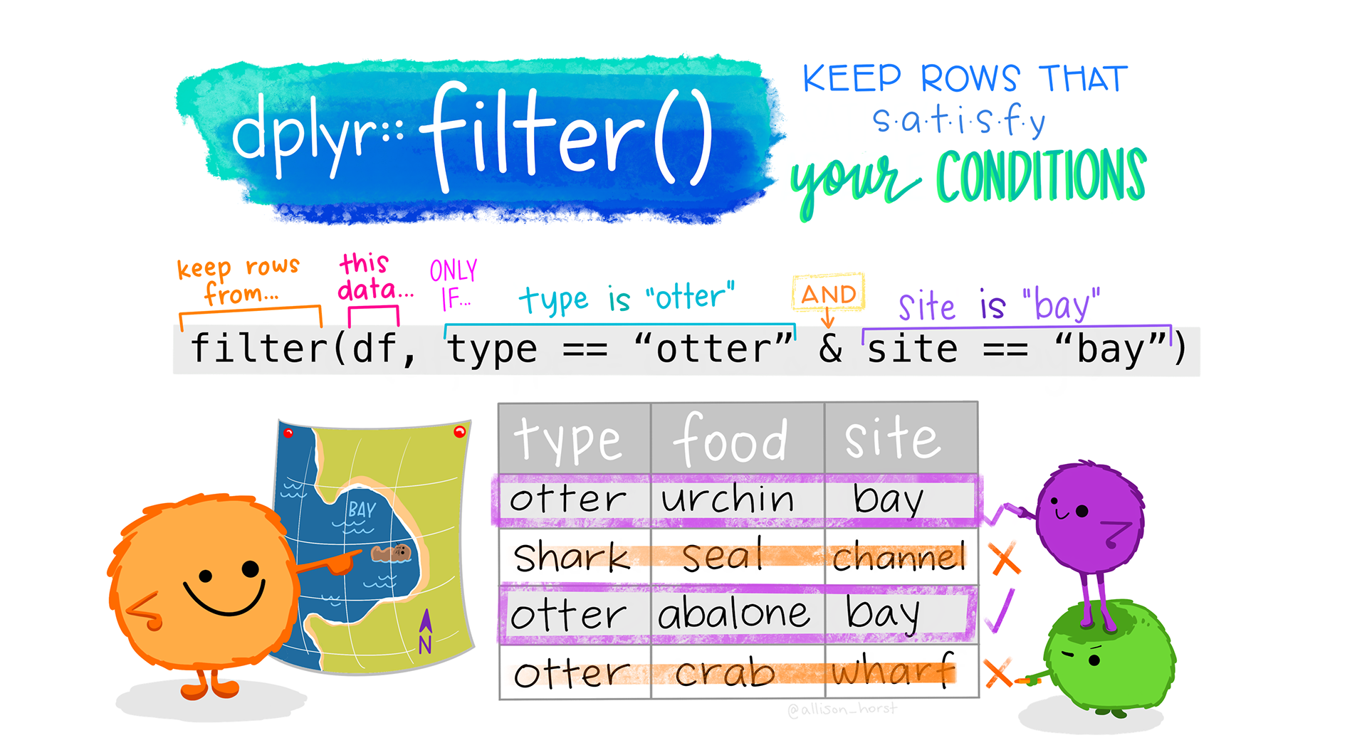
Artwork by Allison Horst

For example, last week we saw how we could filter to countries whose average life expectancy is greater than 80 years old using the following code:

world %>%
  filter(lifeExp >= 80)

Similarly, we might want to filter data based on its spatial relationships. In this case, we use spatial subsetting which is the process of converting a spatial object into a new object containing only the spatial features that relate in space to another object. This is analogous the attribute subsetting that we covered last week (example above).

Topological relationships

When filtering based on attributes, we use conditions (for example, lifeExp >= 80). In spatial subsetting, we use the relationships of objects to each other in space (topological relationships). These relationships are based on mathematical relationships, but can be more easily understood from visualizing them. The figure below shows how each relationship is satisfied.

Geocomputation with R

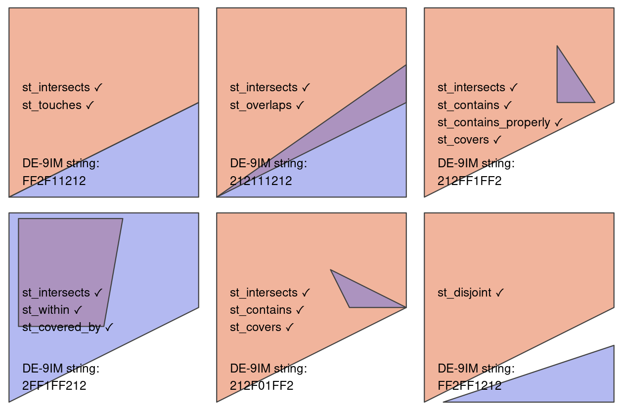
Tipst_intersects() and st_disjoint()

Note that st_intersects()is a “catch-all” that contains the following relationships:

• st_touches()
• st_overlaps()
• st_contains() and st_contains_properly()
• st_covers() and st_covered_by()
• st_within()

st_disjoint() is the opposite of st_intersects()

Examples

There are many ways to spatially subset in R, so we will explore a few.

As an example we’ll work with the following two datasets from the spData package:

• nz: polygons representing the 16 regions of New Zealand
• nz_height: top 101 highest points in New Zealand

We’ll explore by trying to find all the high points in the region of Canterbury (shown in dark grey).

tm_shape(nz) +
  tm_polygons() +
tm_shape(canterbury) +
  tm_polygons(fill = "darkgrey") +
tm_shape(nz_height) +
  tm_dots(fill = "red")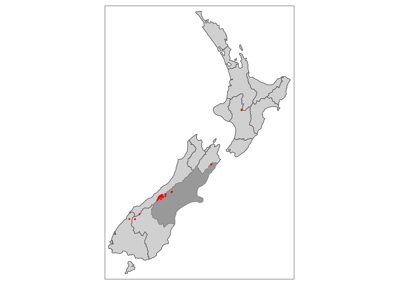

Bracket subsetting

Like attribute subsetting, the command x[y, ] (equivalent to nz_height[canterbury, ]) subsets features of a target x using the contents of a source object y. Instead of y being a vector of class logical or integer, however, for spatial subsetting both x and y must be geographic objects. Specifically, objects used for spatial subsetting in this way must have the class sf or sfc: both nz and nz_height are geographic vector data frames and have the class sf, and the result of the operation returns another sf object representing the features in the target nz_height object that intersect with (in this case high points that are located within) the Canterbury region.

# subset nz_heights to just the features that intersect Canterbury
c_height1 <- nz_height[canterbury, ]

By default bracket subsetting will filter to features in x that intersect features in y. However, we can use other topological relationships by changing options.

nz_height[canterbury, , op = st_disjoint]

st_filter()

The sf package also includes the function st_filter() which is analogous to dplyr::filter(). Using st_filter() we can perform spatial subsetting in the same format as using dplyr commands. The .predicate = argument allows us to define which topological relationship we would like to filter by (e.g. st_intersects(), st_disjoint()).

The results from this method are the identical to the method above.

# subset to the features in Cantebury
c_height2 <- nz_height %>%
  st_filter(y = canterbury, .predicate = st_intersects) # define the topological relationship

Topological operators (st_intersects())

The previous two methods either by default or explicitly use the argument st_intersects. All topological relationships have their own topological operators which are functions that evaluate whether or not features meet the specified condition (e.g. st_intersects()). These operators can be used for spatial subsetting, but are more complicated to use.

The output of st_intersects() and other topological operators is a sparse geometry binary predicate list (yikes!) that’s a list that defines whether or not each feature in x intersects y.

This can be converted into logical vector of TRUE and FALSE values which can then be used for filtering.

# sparse binary predicate list
nz_height_sgbp <- st_intersects(x = nz_height, y = canterbury)
nz_height_sgbp

Sparse geometry binary predicate list of length 101, where the
predicate was `intersects'
first 10 elements:
 1: (empty)
 2: (empty)
 3: (empty)
 4: (empty)
 5: 1
 6: 1
 7: 1
 8: 1
 9: 1
 10: 1

# convert to logical vector
nz_height_logical <- lengths(nz_height_sgbp) > 0

# filter based on logical vector
c_height3 = nz_height[nz_height_logical, ]

Now let’s plot results from all three methods to confirm they gave the same results.

map1 <- tm_shape(nz) +
  tm_polygons() +
  tm_shape(canterbury) +
  tm_fill(fill = "darkgrey") +
  tm_shape(c_height1) +
  tm_dots(fill = "red") +
  tm_title(text = "Bracket subsetting")+ 
  tm_layout(meta.margins = c(.2, 0, 0, 0))

map2 <- tm_shape(nz) +
  tm_polygons() +
  tm_shape(canterbury) +
  tm_fill(fill = "darkgrey") +
  tm_shape(c_height2) +
  tm_dots(fill = "red") +
  tm_title(text = "st_filter()")+ 
  tm_layout(meta.margins = c(.2, 0, 0, 0))

map3 <- tm_shape(nz) +
  tm_polygons() +
  tm_shape(canterbury) +
  tm_fill(fill = "darkgrey") +
  tm_shape(c_height3) +
  tm_dots(fill = "red") +
  tm_title(text = "st_intersects()")+ 
  tm_layout(meta.margins = c(.2, 0, 0, 0))

tmap_arrange(map1, map2, map3, nrow = 1)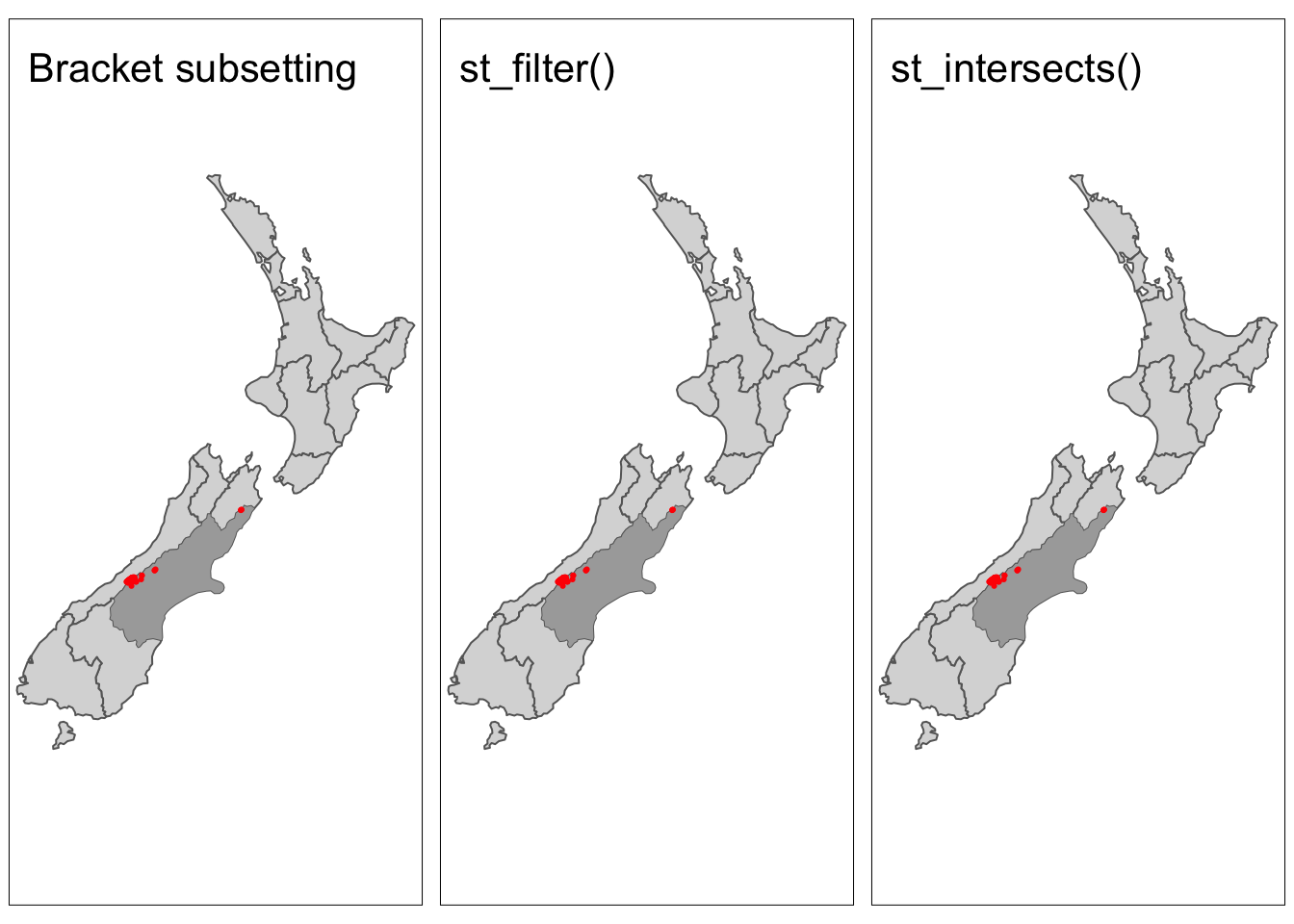

Distance relationships

The topological relationships we have been discussing are all binary (features either intersect or don’t). In some cases, it might be helpful to subset based on a distance to a feature. In these cases we can use the st_is_within_distance() to filter features. By default st_is_within_distance() will return a sparse geometry binary predicate list as in st_intersects() above. Instead, we can return a logical by setting sparse = FALSE.

# find heights within 1000 km of Canterbury
nz_height_logical <- st_is_within_distance(nz_height, canterbury,
                      dist = units::set_units(1000, "km"), # set distance
                      sparse = FALSE) # return logical vector instead

c_height4 <- nz_height[nz_height_logical, ] # filter based on logical

Now, we should see points appear that do not intersect Caterbury, but are within 1000 km.

# additional high points should appear
tm_shape(nz) +
  tm_polygons() +
  tm_shape(canterbury) +
  tm_fill(fill = "darkgrey") +
  tm_shape(c_height4) +
  tm_dots(fill = "red")

3. Spatial joins

Joins are a common way to link different data sources. Up until now, we have been performing joins using common attributes between data.frames. Last week, we saw that the same joins can be used on sf objects. However, we can also perform joins by using the spatial relationship of datasets.

First, let’s remind ourselves of the different types of joins.

Software Carpentry

Toplogical relationships

With spatial data, we can join based on the geometry columns using topological relationships using the st_join() function. By default st_join() will join based on geometries that intersect, but can accommodate other topological relationships by changing the join = argument. By default st_join() performs left joins, but can perform inner joins by setting left = FALSE.

# specify join based on geometries x within y
st_join(x, y, join = st_within)

# specify inner join
st_join(x, y, left = FALSE)

Let’s consider the scenario where we would like to know which region each of the highest points is located in. We can left join the nz dataset (polygons of NZ’s regions) onto the nz_height dataset (points of highest points in the county).

nz_height_left_join <- st_join(nz_height, nz) %>%
  select(id = t50_fid, elevation, region = Name)

head(nz_height_left_join)

Simple feature collection with 6 features and 3 fields
Geometry type: POINT
Dimension:     XY
Bounding box:  xmin: 1204143 ymin: 5048309 xmax: 1389460 ymax: 5168749
Projected CRS: NZGD2000 / New Zealand Transverse Mercator 2000
       id elevation     region                geometry
1 2353944      2723  Southland POINT (1204143 5049971)
2 2354404      2820      Otago POINT (1234725 5048309)
3 2354405      2830      Otago POINT (1235915 5048745)
4 2369113      3033 West Coast POINT (1259702 5076570)
5 2362630      2749 Canterbury POINT (1378170 5158491)
6 2362814      2822 Canterbury POINT (1389460 5168749)

Now we could use this data to summarize the number of highest point in each region!

nz_height_left_join %>%
  group_by(region) %>%
  summarise(n_points = n()) %>%
  st_drop_geometry()

# A tibble: 7 × 2
  region            n_points
* <chr>                <int>
1 Canterbury              70
2 Manawatu-Wanganui        2
3 Marlborough              1
4 Otago                    2
5 Southland                1
6 Waikato                  3
7 West Coast              22

Distance-based joins

Similar to filtering, in some cases we may want to join datasets based on their proximity. Let’s see an example!

We’ll use the following two datasets from the spData package:

• cycle_hire: points representing cycle hire points across London with information on number of bikes available
• cycle_hire_osm: dataset downloaded from OpenStreetMaps representing cycle hire points across London with information on the capacity of the hire point

In this example, we would like join the capacity attribute from the cycle_hire_osm dataset to the cycle_hire dataset. Unfortunately it appears that the points from the two datasets do not perfectly align.

# check whether or not points overlap
if(any(st_intersects(cycle_hire, cycle_hire_osm, sparse = FALSE)) == TRUE){
  print("points overlap")
} else{
  warning("points don't overlap")
}

Warning: points don't overlap

tmap_mode("view")

tm_shape(cycle_hire) +
  tm_symbols(fill = "red" , fill_alpha = 0.2)+
tm_shape(cycle_hire_osm) +
  tm_symbols(fill = "blue", fill_alpha = 0.2)

We can join by again using st_join(), but this time including a distance threshold using st_is_within_distance.

cycle_hire_join <- st_join(cycle_hire, cycle_hire_osm,
                           st_is_within_distance,
                           dist = units::set_units(20, "m")) %>%
                   select(id, capacity)

head(cycle_hire_join)

Simple feature collection with 6 features and 2 fields
Geometry type: POINT
Dimension:     XY
Bounding box:  xmin: -0.1975742 ymin: 51.49313 xmax: -0.08460569 ymax: 51.53006
Geodetic CRS:  WGS 84
  id capacity                     geometry
1  1        9  POINT (-0.1099705 51.52916)
2  2       27  POINT (-0.1975742 51.49961)
3  3       NA POINT (-0.08460569 51.52128)
4  4       NA  POINT (-0.1209737 51.53006)
5  5       NA   POINT (-0.156876 51.49313)
6  6        8  POINT (-0.1442289 51.51812)

Let’s build some checks to diagnose the output.

if(nrow(cycle_hire) == nrow(cycle_hire_join)){
  print("join matches original data dimensions")
} else {
  warning("join does not match orginal data dimensions")
  print(paste("cycle_hire has", nrow(cycle_hire), "rows"))
  print(paste("cycle_hire_join has", nrow(cycle_hire_join), "rows"))
}

Warning: join does not match orginal data dimensions

[1] "cycle_hire has 742 rows"
[1] "cycle_hire_join has 762 rows"

Note that the joined result has more rows than the target data. This is because some of the cycle hire stations in cycle_hire have multiple matches in cycle_hire_osm. Depending on your project, you would need to think about how to resolve this. In this case, we can aggregate the values for the overlapping points by taking the mean.

# aggregate values for single points in cycle_hire
cycle_hire_join <- cycle_hire_join %>%
  group_by(id) %>%
  summarise(capacity = mean(capacity))

# check results
if(nrow(cycle_hire) == nrow(cycle_hire_join)){
  print("join matches original data dimensions")
} else {
  warning("join does not match orginal data dimensions")
  print(paste("cycle_hire has", nrow(cycle_hire), "rows"))
  print(paste("cycle_hire_join has", nrow(cycle_hire_join), "rows"))
}

[1] "join matches original data dimensions"

4. Spatial aggregation

As with aggregating attribute data, spatial data aggregation condenses data: outputs have few rows than inputs. Think about our friend group_by() %>% summarise()! Spatial aggregation is the same.

Let’s consider the example where we would like to make a map of the mean elevation of high points within each region of NZ. There are several ways to do this, but the first thing we should be thinking is that we will need to retain the geometry column of the NZ regions in order to make a map.

The first approach is by leveraging st_join() again. But in this example, we want the nz object to be the target to maintain the geometries we need.

tmap_mode("plot")

ℹ tmap mode set to "plot".

nz_elevation <- st_join(x = nz, y = nz_height) %>%
  group_by(Name) %>%
  summarise(elevation = mean(elevation, na.rm = TRUE))

The second approah uses the aggregate() function. Although it doesn’t follow the dplyr piping convention we’re used to, aggregate() will come in handy later, so it’s nice to see how it works.

The syntax looks slightly different, in this case the argument x is the data we would like to aggregate (nz_height) and the by argument specifies the geometry that you would like to group by. The FUN argument defines the function that you would like to use to aggregate, in this case mean.

nz_elevation <- aggregate(x = nz_height, by = nz, FUN = mean)

map1 <- tm_shape(nz_elevation) +
  tm_polygons(fill = "elevation",
              fill.legend= tm_legend(title = "Mean elevation (meters)")) +
  tm_title(text = "group_by()")+ 
  tm_layout(meta.margins = c(.2, 0, 0, 0))

map2 <- tm_shape(nz_elevation) +
  tm_polygons(fill = "elevation",
              fill.legend = tm_legend(title = "Mean elevation (meters)")) +
  tm_title(text = "aggregate()")+ 
  tm_layout(meta.margins = c(.2, 0, 0, 0))

tmap_arrange(map1, map2, nrow = 1)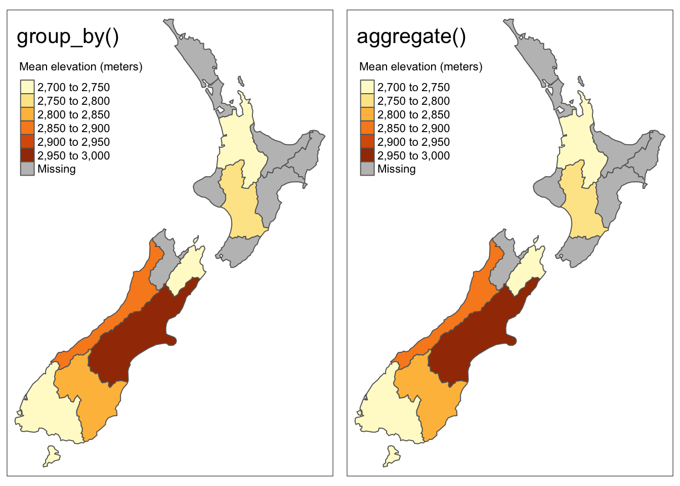

NoteJoining incongruent layers

An important consideration when aggregating spatial objects is that geometries are congruent, meaning aggregating zones align with the units being aggregating. This is often the case with administrative boundaries where units are sub-units of one another (e.g. countries > states > counties).

However, in some cases the aggregating zones do not share common borders with the target. This is an issue because it’s not clear how to aggregate underlying data. Areal interpolation overcomes this issue by transferring values to another using algorithms, including simple area weighted approaches.

incongruent <- spData::incongruent
aggregating_zones <- spData::aggregating_zones

tm_shape(incongruent) +
  tm_polygons(fill = "lightblue",
              col = "blue") +
  tm_shape(aggregating_zones) +
  tm_borders(col = "red")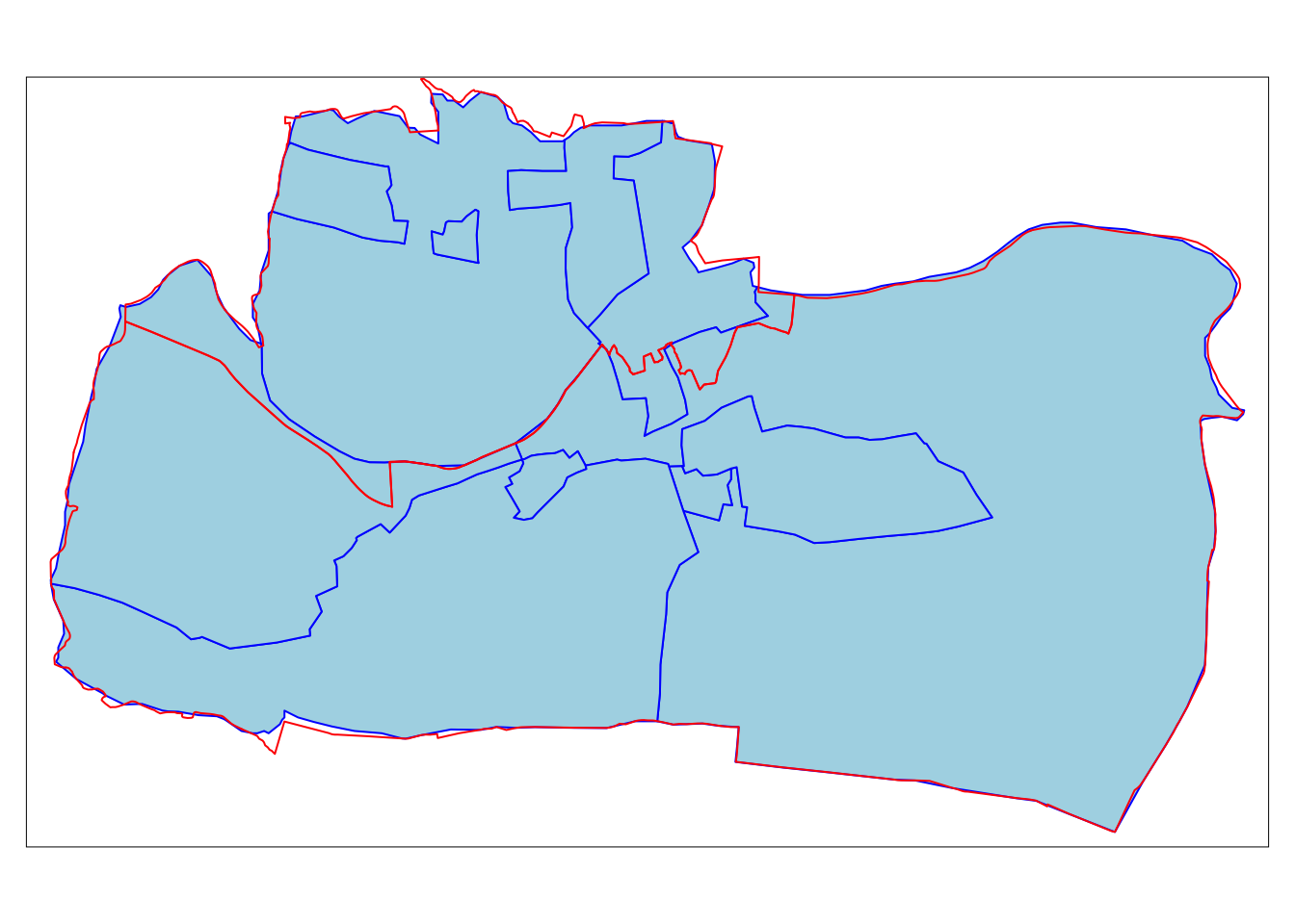

The simplest useful method for this is area weighted spatial interpolation, which transfers values from the incongruent object to a new column in aggregating_zones in proportion with the area of overlap: the larger the spatial intersection between input and output features, the larger the corresponding value. This is implemented in st_interpolate_aw(), as demonstrated in the code chunk below.

# select just the value to be aggregated
incongruent_2 <- incongruent %>%
  select(value)

# use area-weighted interpolation to aggregrate the "value" attribute
aggregating_zones_area_weighted <- st_interpolate_aw(incongruent_2, aggregating_zones, extensive = TRUE)

Warning in st_interpolate_aw.sf(incongruent_2, aggregating_zones, extensive =
TRUE): st_interpolate_aw assumes attributes are constant or uniform over areas
of x

aggregating_zones_area_weighted$value

[1] 19.61613 25.66872

Geometry operations

In the previous section, we saw how we can use spatial relationship of datasets to perform operations. We did so by leveraging the geometry columnn, but none of our operations changed the underlying geometries – mapping our output produces the same objects.

In this section, we will explore operations that change the geometries directly.

1. Aggregating

Geometry unions

We may come across situations where we would like to summarize data across several spatial units. For example, summarizing the population across states within regions of the US. Based on our experience with tabular data, we can summarize attributes by using group_by() %>% summarize(). Alternatively we can use the aggregate() function. So far this should look familiar, but if plot the outputs we notice that these functions have also aggregated the underlying geometries.

# load US states
us_states <- spData::us_states

# summarize total population within each region
regions1 <- us_states %>%
  group_by(REGION) %>%
  summarise(population = sum(total_pop_15, na.rm = TRUE))

# alternative approach
regions2 <- aggregate(x = us_states[, "total_pop_15"], # data and attribute to be aggregated
                      by = list(us_states$REGION), # attribute to aggregate by
                      FUN = sum, na.rm = TRUE) # aggregating function

map1 <- tm_shape(us_states) +
  tm_polygons(fill = "total_pop_15",
              fill.legend  = tm_legend("Total population")) +
  tm_title(text = "US States")+
  tm_layout(meta.margins = c(.2, 0, 0, 0))

map2 <- tm_shape(regions1) +
  tm_polygons(fill = "population",
              fill.legend  = tm_legend("Total population")) +
  tm_title(text = "group_by()")+ 
  tm_layout(meta.margins = c(.2, 0, 0, 0))

map3 <- tm_shape(regions2) +
  tm_polygons(fill = "total_pop_15",
              fill.legend  = tm_legend("Total population")) +
  tm_title(text = "aggregate()")+ 
  tm_layout(meta.margins = c(.2, 0, 0, 0))

tmap_arrange(map1, map2, map3, nrow = 1)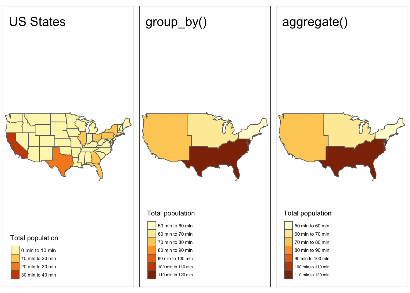

What’s going on here? Behind the scenes, R is using st_union() to combine geometries within each group. We can also use st_union() to combine any pair of spatial objects.

# combine geometries of western states
us_west <- us_states[us_states$REGION == "West", ]
us_west_union <- st_union(us_west)

# combine geometries of Texas and western states
texas <- us_states[us_states$NAME == "Texas", ]
texas_union <- st_union(us_west_union, texas)

map1 <- tm_shape(us_west) +
  tm_polygons() +
  tm_title(text = "western states")+ 
  tm_layout(meta.margins = c(.2, 0, 0, 0))

map2 <- tm_shape(us_west_union) +
  tm_polygons() +
  tm_title(text = "western states union")+ 
  tm_layout(meta.margins = c(.2, 0, 0, 0))

map3 <- tm_shape(texas) +
  tm_polygons() +
  tm_title(text = "TX")+ 
  tm_layout(meta.margins = c(.2, 0, 0, 0))

map4 <- tm_shape(texas_union) +
  tm_polygons() +
  tm_title(text = "TX + western states union")+ 
  tm_layout(meta.margins = c(.2, 0, 0, 0))

tmap_arrange(map1, map2, map3, map4, nrow = 2)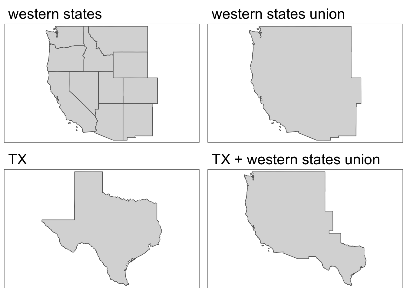

2. Filtering

Buffers

In the previous section, we saw that we can filter spatial objects based on their proximity using st_is_within_distance(). An alternative approach to finding items that are within a set distance would be to expand the geometry and then intersect with objects of interest. We can change the size of geometries by creating a “buffer” using st_buffer()

In this example, let’s create 5 km and 50 km buffers around the Seine.

seine_buffer_5km <- st_buffer(seine, dist = 5000)
seine_buffer_50km = st_buffer(seine, dist = 50000)

map1 <- tm_shape(seine_buffer_5km) +
  tm_polygons() +
  tm_shape(seine) +
  tm_lines() +
  tm_title(text = "5km buffer")+ 
  tm_layout(meta.margins = c(.2, 0, 0, 0))

map2 <- tm_shape(seine_buffer_50km) +
  tm_polygons() +
  tm_shape(seine) +
  tm_lines() +
  tm_title(text = "50km buffer")+ 
  tm_layout(meta.margins = c(.2, 0, 0, 0))

tmap_arrange(map1, map2, nrow = 1)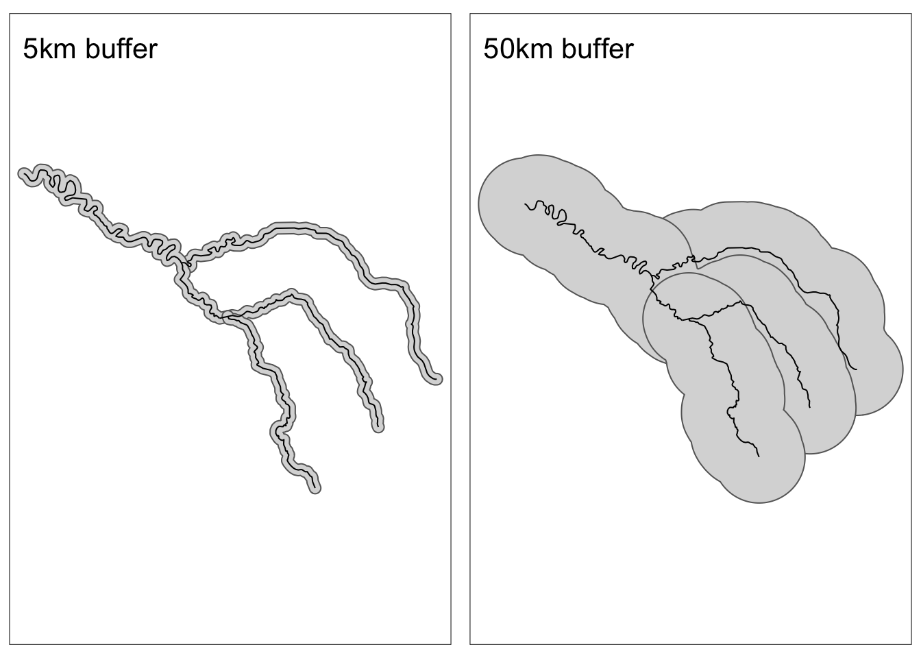

The Seine is actually comprised of multiple geometries. To make things simpler, and more look better on maps, we can combine geometries using our new friend st_union!

seine_union <- st_union(seine_buffer_50km)

tm_shape(seine_union) +
  tm_polygons() +
  tm_shape(seine) +
  tm_lines() +
  tm_title(text= "50km buffer")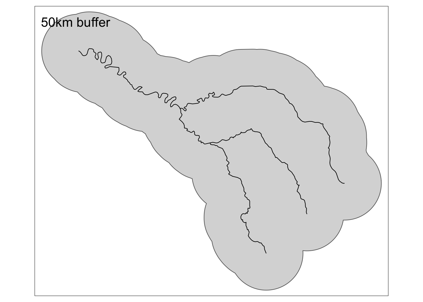

Now let’s see an example of using a buffer to find objects within a set distance. Here, we’ll repeat our previous example of finding points within 100 km of Canterbury. And check to see if the results match our previous approach!

# create buffer around high points
nz_height_buffer <- st_buffer(nz_height, dist = 1000000)

# filter buffered points with those that intersect Canterbury
c_height5 <- nz_height_buffer %>%
  st_filter(y = canterbury, .predicate = st_intersects)

# check to see if results match previous approach
if(nrow(c_height4) == nrow(c_height5)){
  print("results from buffer approach match st_is_within_distance() approach")
} else{
  warning("approaches giving different results")
}

[1] "results from buffer approach match st_is_within_distance() approach"

Clipping

Beyond filtering observations based on their spatial proximity, in some cases we might want to filter (or remove) portions of geometries. Spatial clipping is a form of spatial subsetting that involves changes to the geometry columns of at least some of the affected features.

Clipping can only apply to features more complex than points: lines, polygons and their ‘multi’ equivalents.

There are several options for clipping geometries:

• st_intersection(x, y) - portion of x intersecting y
• st_difference(x, y) - portion of x not intersecting y
• st_difference(y, x) - portion of y not intersecting x
• st_union(x, y) - portion either in x or y
• st_sym_difference(x, y) - portions of x and y that do not intersect

To illustrate the concept, we will start with a simple example: two overlapping circles with a center point one unit away from each other and a radius of one.

x <- st_sfc(st_point(c(0, 1))) %>%
  st_buffer(dist = 1) %>%
  st_sf() 

y <- st_sfc(st_point(c(1, 1))) %>%
  st_buffer(dist = 1) %>%
  st_sf()

intersection <- st_intersection(x, y) 
difference_x_y <- st_difference(x, y) 
difference_y_x <- st_difference(y, x)
union <- st_union(x, y)
sym_difference <- st_sym_difference(x, y) 

x <- x %>% st_set_crs(4326)
y <- y %>% st_set_crs(4326)
bbox <- st_union(x, y)

map1 <- tm_shape(x, bbox = bbox) +
  tm_borders(col = "red") +
  tm_shape(y) +
  tm_borders(col = "blue")+ 
  tm_layout(meta.margins = c(.2, 0, 0, 0))

map2 <- map1 +
  tm_shape(intersection, bbox = bbox) +
  tm_fill(col = "purple") +
  tm_title(text = "st_intersection()")+ 
  tm_layout(meta.margins = c(.2, 0, 0, 0))

map3 <- map1 +
  tm_shape(difference_x_y, bbox = bbox) +
  tm_fill(col = "purple") +
  tm_title(text = "st_difference(x,y)")+ 
  tm_layout(meta.margins = c(.2, 0, 0, 0))


map4 <- map1 +
  tm_shape(difference_y_x, bbox = bbox) +
  tm_fill(col = "purple") +
  tm_title(text = "st_difference(y,x)")+
  tm_layout(meta.margins = c(.2, 0, 0, 0))

map5 <- map1 +
  tm_shape(union, bbox = bbox) +
  tm_fill(col = "purple") +
  tm_title(text = "st_union()")+ 
  tm_layout(meta.margins = c(.2, 0, 0, 0))

map6 <- map1 +
  tm_shape(sym_difference, bbox = bbox) +
  tm_fill(col = "purple") +
  tm_title(text = "st_sym_diffference()")+ 
  tm_layout(meta.margins = c(.2, 0, 0, 0))

tmap_arrange(map1, map2, map3, map4, map5, map6, nrow = 2)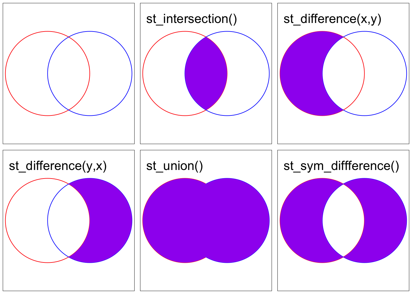

Now let’s see how we could use these updated geometries for filtering. Extending this simple example, we’ll create 100 random points. We want to find the points that intersect both x and y. We have a few different approaches that all produce the same results.

# create random points
bb <- st_bbox(bbox) # create bounding box of x and y
box <- st_as_sfc(bb)
p <- st_sample(x = box, size = 100) %>% # randomly sample the bounding box
  st_as_sf()

# find intersection of x and y
x_and_y <- st_intersection(x, y)
x_and_y <- st_make_valid(x_and_y)


# filter points
# first approach: bracket subsetting
p_xy1 = p[x_and_y, ]

# second approach: st_filter()
p_xy2 <- p %>%
  st_filter(., x_and_y)

# third approach: st_intersection()
p_xy3 = st_intersection(p, x_and_y)

map2 <- map1 +
  tm_shape(p) +
  tm_dots(alpha = 0.5) +
  tm_layout(main.title = "original")

map3 <- map2 +
  tm_shape(p_xy1) +
  tm_symbols(col = "purple", size = 0.2) +
  tm_layout(main.title = "bracket subsetting")

map4 <- map2 +
  tm_shape(p_xy2) +
  tm_symbols(col = "purple", size = 0.2) +
  tm_layout(main.title = "st_filter()")

map5 <- map2 +
  tm_shape(p_xy3) +
  tm_symbols(col = "purple", size = 0.2) +
  tm_layout(main.title = "st_intersection()")

tmap_arrange(map2, map3, map4, map5, nrow = 2)

3. Making life easier!

Working with, and especially plotting, complex spatial objects can become quite cumbersome. This section we’ll see a few ways to create and manipulate geometries to make them easier to work with.

Centroids

Centroids are basically the center of spatial objects. They can be a handy way to display summary statistics (or we might actually use them for analysis – e.g. to find the distance between polygons).

There are many ways to that we might want to define the “center” of an object, but the most common is the geographic centroid which is the center of mass of a spatial object. The geographic centroid can be found using st_centroid().

Sometimes the geographic centroid may fall outside of the boundaries of the object (picture the centroid of a doughnut!). While correct, it might be confusing on a map, so we can use st_point_on_surface() to ensure that the centroid is placed onto the object.

Let’s inspect a few examples!

nz_centroid <- st_centroid(nz)
seine_centroid <- st_centroid(seine)

nz_pos <- st_point_on_surface(nz)
seine_pos <- st_point_on_surface(seine)

map1 <- tm_shape(nz) +
  tm_polygons() +
  tm_shape(nz_centroid) +
  tm_symbols(fill = "red", fill_alpha = 0.5) +
  tm_shape(nz_pos) +
  tm_symbols(fill = "blue", fill_alpha = 0.5)+ 
  tm_layout(meta.margins = c(.2, 0, 0, 0))

map2 <- tm_shape(seine) +
  tm_lines() +
  tm_shape(seine_centroid) +
  tm_symbols(fill = "red", fill_alpha = 0.5) +
  tm_shape(seine_pos) +
  tm_symbols(fill = "blue", fill_alpha = 0.5)+ 
  tm_layout(meta.margins = c(.2, 0, 0, 0))

tmap_arrange(map1, map2, nrow = 1)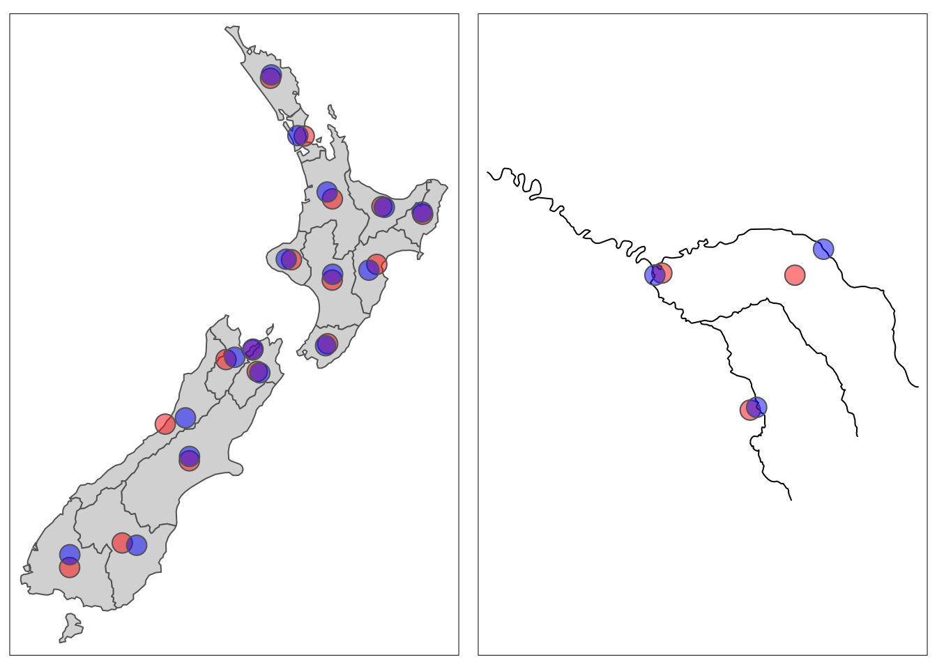

Simplification

We may also want to simplify a geometry to make it easier to plot or take up less storage. There are several different algorithms for simplifying geometries, check out Geocomputation with R for more examples. The sf packages uses the Douglas-Peucker algorithm within the st_simplify() function.

Let’s see an example!

seine_simple <- st_simplify(seine, dTolerance = 2000)  # 2000 m

map1 <- tm_shape(seine) +
  tm_lines() +
  tm_title("original")+ 
  tm_layout(meta.margins = c(.2, 0, 0, 0))

map2 <- tm_shape(seine_simple) +
  tm_lines() +
  tm_title("st_simplify()")+ 
  tm_layout(meta.margins = c(.2, 0, 0, 0))

tmap_arrange(map1, map2, nrow = 1)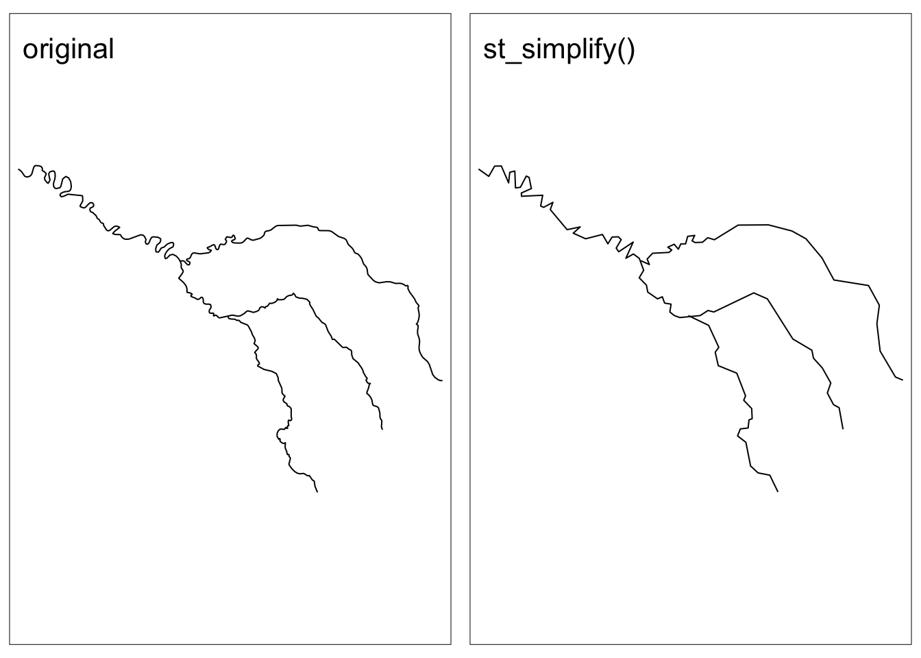

Summary of new functions

Brief description of new functions, check out documentation for more information

Function	Description
Spatial data operations
st_intersects(x,y)	tests whether objects intersects
st_touches(x,y)	tests whether objects touch
st_overlaps(x,y)	tests whether objects overlap
st_contains(x,y)	tests whether object x contains object y (including boundary)
st_contains_properly(x,y)	tests whether object x contains object y (not including boundary)
st_covers(x,y)	identical to st_contains() when y is a polygon
st_covered_by(x,y)	tests whether object y contains object x
st_within(x,y)	tests whether object x is within object y
st_disjoint(x,y)	tests whether objects have no intersection
st_is_within_distance(x,y)	test whether objects intersect within a certain distance
st_join(x,y)	performs spatial join
st_interpolate_aw(x,y)	performs area-weighted interpolation of polygons
Geometry operations
aggregate(x,y)	computes summary statistics for data subsets
st_union(x,y)	combines geometries
st_buffer(x)	creates polygon that represents all points within a distance threshold of original geometry
st_intersection(x,y)	creates polygon of the area shared by x and y
st_difference(x,y)	creates polygon of the area of x not in y
st_sym_difference(x,y)	creates polygon of the area not shared by x and y
st_centroid(x)	creates point(s) of the geographic centroid of a polygon(s)
st_simplify(x)	creates a simplified representation of a geometry