Week 8: Discussion Section

Santa Clara River — The Nature Conservancy

Source Materials

The following materials are based on materials developed by Dr. Chris Kibler for the UCSB Geography Department.

Phenology is the timing of life history events. Important phenological events for plants involve the growth of leaves, flowering, and senescence (death of leaves). Plants species adapt the timing of these events to local climate conditions to ensure successful reproduction. Subsequently, animal species often adapt their phenology to take advantage of food availability. As the climate shifts this synchronization is being thrown out of whack. Shifts in phenology are therefore a common yardstick of understanding how and if ecosystems are adjusting to climate change.

Plant species may employ the following phenological strategies:

Winter deciduous: lose leaves in the winter, grow new leaves in the spring
Drought deciduous: lose leaves in the summer when water is limited
Evergreen: maintain leaves year-round

Learning objectives

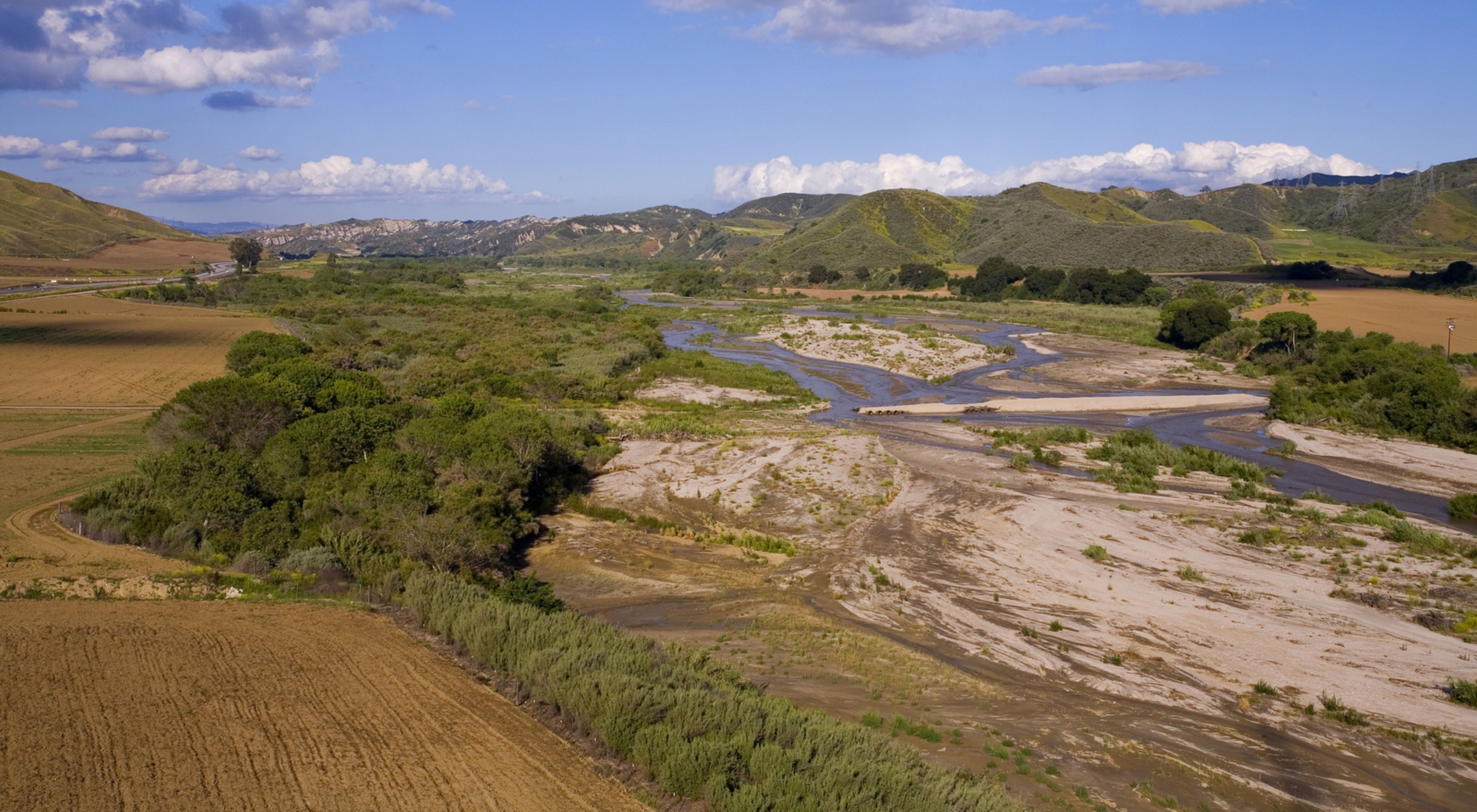
In this lab we are analyzing plant phenology near the Santa Clara River which flows from Santa Clarita to Ventura. We will investigate the phenology of the following plant communities:

Riparian forests: grow along the river, dominated by winter deciduous cottonwood and willow trees
Grasslands: grow in openspaces, dominated by drought deciduous grasses
Chaparral shrublands: grow in more arid habitats, dominated by evergreen shrubs

To investigate the phenology of these plant communities we will use a time series of Landsat imagery and polygons identifying the locations of study sites within each plant community.

Our primary goal is to compare seasonal patterns across vegetation communities. To do so, we will:

Convert spectral reflectance into a measure of vegetation productivity (NDVI)
Calculate NDVI throughout the year
Summarize NDVI values within vegetation communities
Visualize changes in NDVI within vegetation communities

1. Get started

Create a version-controlled R Project
Add (at least) a subfolder to your R project: data
Create a Quarto document

Let’s load all necessary packages:

library(terra)
library(sf)
library(tidyverse)
library(here)
library(tmap)

You will be working with the following datasets:

Multi-spectral remote sensing data: Landsat’s Operational Land Imager (OLI)

8 pre-processed scenes
- Level 2 surface reflectance products
- Erroneous values set to NA
- Scale factor set to 100
- Bands 2-7
- Dates in file name
Scenes from the following dates:
- 2018-06-12
- 2018-08-15
- 2018-10-18
- 2018-11-03
- 2019-01-22
- 2019-02-23
- 2019-04-12
- 2019-07-01

Locations of representative vegetation communities: Polygons representing sites

study_site: character string with plant type

Next, let’s download our data. Unzip and move this to your version-controlled R Project’s data folder.

Create function to compute NDVI

Let’s start by defining a function to compute the Normalized Difference Vegetation Index (NDVI). NDVI computes the difference in reflectance between the near infrared (NIR) and red bands, normalized by their sum.

ndvi_fun <- function(nir, red){
  (nir - red) / (nir + red)
}

Compute NDVI for a single scene

We have 8 scenes collected by Landsat’s OLI sensor on 8 different days throughout the year.

Let’s start by loading in the first scene collected on June 12, 2018:

landsat_20180612 <- rast(here("data", "landsat_20180612.tif"))

Let’s update the names of the layers to match the spectral bands they correspond to:

names(landsat_20180612) <- c("blue", "green", "red", "NIR", "SWIR1", "SWIR2")

Now we can apply the NDVI function we created to compute NDVI for this scene using the lapp() function.

The lapp() function applies a function to each cell using layers as arguments.
Therefore, we need to tell lapp() which layers (or bands) to pass into the function.

The NIR band is the 4th layer and the red band is the 3rd layer in our raster. In this case, because we defined the NIR band as the first argument and the red band as the second argument in our function, we tell lapp() to use the 4th layer first and 3rd layer second.

ndvi_20180612 <- lapp(landsat_20180612[[c(4, 3)]], fun = ndvi_fun)

Code

tm_shape(ndvi_20180612) +
  tm_raster(col.legend  = tm_legend("NDVI")) +
  tm_layout(legend.outside.position = "right")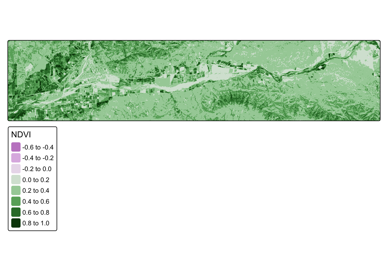

Compute NDVI for all scences

Now we want to repeat the same operations for all 8 scenes. Below is a solution (where we repeat each line for each scene), but it’s pretty clunky.

landsat_20180612 <-rast(here( "data", "landsat_20180612.tif"))
landsat_20180815 <- rast(here("data", "landsat_20180815.tif"))
landsat_20181018 <- rast(here("data", "landsat_20181018.tif"))
landsat_20181103 <- rast(here("data", "landsat_20181103.tif"))
landsat_20190122 <- rast(here("data", "landsat_20190122.tif"))
landsat_20190223 <- rast(here("data", "landsat_20190223.tif"))
landsat_20190412 <- rast(here("data", "landsat_20190412.tif"))
landsat_20190701 <- rast(here("data", "landsat_20190701.tif"))

And rename each layer:

names(landsat_20180612) <- c("blue", "green", "red", "NIR", "SWIR1", "SWIR2")
names(landsat_20180815) <- c("blue", "green", "red", "NIR", "SWIR1", "SWIR2")
names(landsat_20181018) <- c("blue", "green", "red", "NIR", "SWIR1", "SWIR2")
names(landsat_20181103) <- c("blue", "green", "red", "NIR", "SWIR1", "SWIR2")
names(landsat_20190122) <- c("blue", "green", "red", "NIR", "SWIR1", "SWIR2")
names(landsat_20190223) <- c("blue", "green", "red", "NIR", "SWIR1", "SWIR2")
names(landsat_20190412) <- c("blue", "green", "red", "NIR", "SWIR1", "SWIR2")
names(landsat_20190701) <- c("blue", "green", "red", "NIR", "SWIR1", "SWIR2")

Next, compute NDVI for each layer:

ndvi_20180612 <- lapp(landsat_20180612[[c(4, 3)]], fun = ndvi_fun)
ndvi_20180815 <- lapp(landsat_20180815[[c(4, 3)]], fun = ndvi_fun)
ndvi_20181018 <- lapp(landsat_20181018[[c(4, 3)]], fun = ndvi_fun)
ndvi_20181103 <- lapp(landsat_20181103[[c(4, 3)]], fun = ndvi_fun)
ndvi_20190122 <- lapp(landsat_20190122[[c(4, 3)]], fun = ndvi_fun)
ndvi_20190223 <- lapp(landsat_20190223[[c(4, 3)]], fun = ndvi_fun)
ndvi_20190412 <- lapp(landsat_20190412[[c(4, 3)]], fun = ndvi_fun)
ndvi_20190701 <- lapp(landsat_20190701[[c(4, 3)]], fun = ndvi_fun)

Let’s combine NDVI layers into a single raster stack.

all_ndvi <- c(ndvi_20180612, 
              ndvi_20180815, 
              ndvi_20181018, 
              ndvi_20181103, 
              ndvi_20190122, 
              ndvi_20190223, 
              ndvi_20190412, 
              ndvi_20190701)

Now, update the names of each layer to match the date of each image:

names(all_ndvi) <- c("2018-06-12", 
                     "2018-08-15", 
                     "2018-10-18", 
                     "2018-11-03", 
                     "2019-01-22", 
                     "2019-02-23", 
                     "2019-04-12", 
                     "2019-07-01")

The first attempt was pretty clunky and required a lot of copy/pasting. Because we’re performing the same operations over and over again, this is a good opportunity to generalize our workflow into a function!

When should I create a function?

There are lots and lots of reasons to create a function! The biggest clue that you should consider creating one is if you have several lines of code duplicated.

If you’ve been following along, let’s clear our environment rm(list = ls()and redefine our function for NDVI!

2. Create function to compute NDVI

Let’s define a function for NDVI, which computes the difference in reflectance between the near infrared (NIR) and red bands, normalized by their sum.

Solution

ndvi_fun <- function(nir, red){
  (nir - red) / (nir + red)
}

3. Write pseudo code

Let’s first sketch out what operations we want to perform so we can figure out what our function needs. Before diving into the detailed nuances of your function, it’s helpful to start by outlining the major steps you want your function to perform using pseudo-code.

Solution

# NOTE: this code is not meant to run! 
# We're just outlining the function we want to create

create_ndvi_layer <- function(){
  # step 1: read scene
  landsat <- rast(file)
  # step 2: rename layer
  names(landsat) <- c("blue", "green", "red", "NIR", "SWIR1", "SWIR2")
  # step 3: compute NDVI
  ndvi <- lapp(landsat[[c(4, 3)]], fun = ndvi_fun)
  return(ndvi)
}

# What do we notice as what we need to pass into our function?

Now that we’ve written out the pseudo-code, we need to ask ourselves what argument(s) we would need to pass into our function to set off the process. In this case, the first operation needs a file name to read in. So, we now we need to figure out a way to come up with a set of file names to iterate through.

4. Obtain list of Landsat scenes for NDVI function

We want a list of the scenes so that we can tell our function to compute NDVI for each. To do that we look in our data folder for the relevant file. To do so, we want to do the following:

Ask for the names of all the files in the data folder
Set the pattern option to return the names that end in .tif (the file extension for the Landsat scenes)
Set the full.names option returns the full file path for each scene

Solution

files <- list.files(
  here("data"), pattern = "\\*.tif$",
  full.names = TRUE)

5. Update function to compute NDVI with list

Now let’s update our function to work with list of file names we created:

Pass function a number that will correspond to the index in the list of file names

Solution

create_ndvi_layer <- function(i){
  landsat <- rast(files[i])
  names(landsat) <- c("blue", "green", "red", "NIR", "SWIR1", "SWIR2")
  ndvi <- lapp(landsat[[c(4, 3)]], fun = ndvi_fun)
  return(ndvi)
}

Let’s test our function by asking it to read in the first file:

test <- create_ndvi_layer(1)

6. Compute NDVI for each scene and create raster stack

Now we can use our function to create a NDVI layer for each scene and stack them into a single raster stack. And then update layer names to match date:

Solution

Is there a way to improve this last step even further? Wrap it into a for loop? Could we pull the date strings directly from the file names?

all_ndvi <- c(create_ndvi_layer(1), 
              create_ndvi_layer(2), 
              create_ndvi_layer(3), 
              create_ndvi_layer(4), 
              create_ndvi_layer(5), 
              create_ndvi_layer(6), 
              create_ndvi_layer(7), 
              create_ndvi_layer(8))

names(all_ndvi) <- c("2018-06-12", 
                    "2018-08-15", 
                    "2018-10-18", 
                    "2018-11-03", 
                    "2019-01-22", 
                    "2019-02-23", 
                    "2019-04-12", 
                    "2019-07-01")

7. Compare NDVI across vegetation communities

Now that we have computed NDVI for each of our scenes (days) we want to compare changes in NDVI values across different vegetation communities.

Read shapefile of study sites to obtain data on vegetation communities

sites <- st_read(here("data","study_sites.shp"))

Code

tm_shape(all_ndvi[[1]]) +
  tm_raster() +
  tm_shape(sites) +
  tm_polygons() +
  tm_layout(legend.show = FALSE)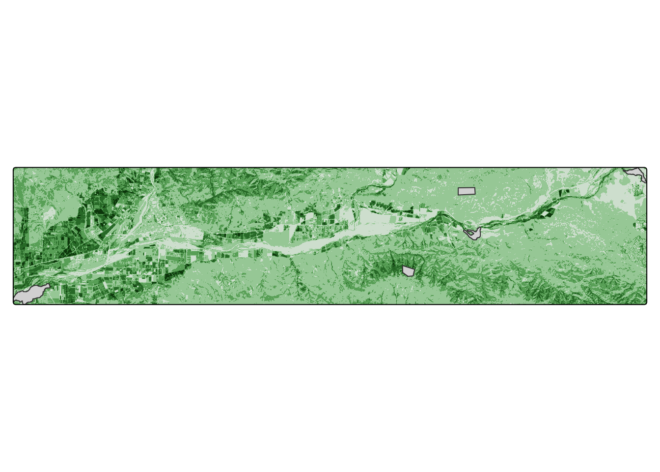

Apply zonal statistics to obtain mean NDVI at study sites

Now we want to find the average NDVI within each study site. The output of terra::zonal() is a data.frame with rows that match the study site data set, so we bind the results to the original data set.

Solution

veg_zones <- rasterize(sites, all_ndvi, field = "study_site")

sites_ndvi <- terra::zonal(all_ndvi, veg_zones, fun = "mean")

sites_annotated <- cbind(sites, sites_ndvi)

sites_ndvi <- terra::extract(all_ndvi, sites, fun = "mean")

sites_annotated <- cbind(sites, sites_ndvi)

8. Tidy data frame

We’re done! Except our data is very untidy… Let’s tidy it up!

Convert to data frame
Turn from wide to long format
Turn layer names into date format
Combine study sites by vegetation type
Summarize results within vegetation types

Solution

sites_clean <- sites_annotated |> 
  # initial cleaning
  st_drop_geometry() |> # drop geometry
  select(-ID) |> # remove ID generated by terra::extract()
  # reformat data frame
  pivot_longer(!study_site) |>  # reshape data frame
  rename("NDVI" = value) |>  # assign "value" to NDVI
  # create date attribute
  mutate("year" = str_sub(name, 2, 5), # pull out elements of date
         "month" = str_sub(name, 7, 8),
         "day" = str_sub(name, -2, -1)) |> 
  unite("date", 4:6, sep = "-") |>  # combine date elements
  mutate("date" = lubridate::as_date(date)) |> 
  # rename combine study sites by vegetation type
  mutate("veg_type" = case_when(study_site == "forest1" ~ "forest",
                                study_site == "forest2" ~ "forest",
                                study_site == "forest3" ~ "forest",
                                study_site == "grassland" ~ "grassland",
                                study_site == "chaparral" ~ "chaparral")) |> 
  # summarize results by vegetation type
  group_by(veg_type, date) |> 
  summarize("NDVI" = mean(NDVI, na.rm = TRUE))

Let’s plot the results!

Code

ggplot(sites_clean,
       aes(x = date, y = NDVI,
           group = veg_type, col = veg_type)) +
  scale_color_manual(values = c("#EAAC8B", "#315C2B","#9EA93F")) +
  geom_line() +
  geom_point() +
  theme_minimal() +
  labs(x = "", y = "Normalized Difference Vegetation Index (NDVI)", col = "Vegetation type",
       title = "Seasonal cycles of vegetation productivity")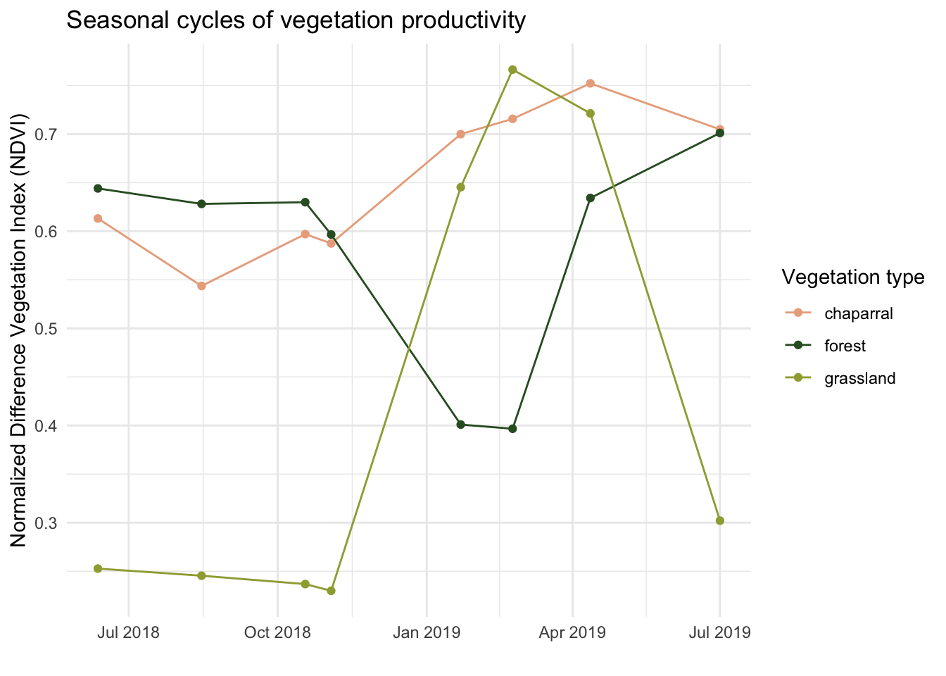

What do we notice in the seasonal cycle in NDVI across vegetation communities?

chaparral: NDVI stays relatively constant throughout the year
forest: NDVI is lowest in the winter and highest in the summer
grassland: NDVI is highest in the winter and lowest in the summer

Does this match our expectations?