Source Materials

The following materials are modified from Geocomputation with R by Robin Lovelace. This page works through the same raster exercises twice: first with terra (Part 1), then with sf and stars (Part 2).

Get Started

Create a version-controlled R Project
Create a Quarto document

Warning

If you don’t have spDataLarge installed, make sure to run:
install.packages('spDataLarge', repos='https://nowosad.github.io/drat/', type='source')

Let’s load all necessary packages:

library(tidyverse)
library(spDataLarge)
library(sf)
library(stars)
library(terra)

You will be working with the following datasets:

Digital elevation model (DEM) of Mt. Mongón, Perú, obtained from spDataLarge
Landsat image of Zion National Park, obtained from spDataLarge
SRTM elevation of Zion National Park, obtained from spDataLarge

Exercises

Explore elevation at Mt. Mongón, Perú
- Make a boxplot and histogram of elevation at Mt. Mongón, Perú
- Reclassify dem and compute the mean for the three classes:
  - Low, where elevation is less than 300
  - Medium
  - High, where elevation is greater than 500
Explore NDVI and NDWI at Zion National Park
- Calculate the Normalized Difference Vegetation Index (NDVI) at Zion National Park
- Calculate the Normalized Difference Water Index (NDWI) at Zion National Park
- Find a correlation between NDVI and NDWI at Zion National Park
Change resolution of elevation at Zion National Park
- Use all the methods available to change the resolution of elevation at Zion National Park to 0.01 by 0.01 degrees
  - Note: The srtm raster has a resolution of 0.00083 by 0.00083 degrees

Landsat 8 bands 2-5 correspond to bands 1-4 for this raster. Bands are as follows:

Band		Color
1	blue	30 meter
2	green	30 meter
3	red	30 meter
4	near-infrared	30 meter

Apply a scale factor and offset for all grid cells

Landsat Level-2 products are written as scaled integers to allow us to convert the data from floating point to integer for delivery. In most cases these are written to a 16-bit integer, which saves disk space and provides faster download times. Each floating point pixel has an offset applied and then multiplied by a gain to bring the value into the 16-bit integer (or unsigned integer) range. These values are referred to as scaled integers. To allow the user to get the data back to its original floating point value, a scale factor and offset are provided for each band.

Science product	Scale factor	Offset
Surface reflectance	0.0000275	-0.2

First, correct the scale across all grid cells and then apply the following functions at each grid cell, in the image:

\[\text{NDWI} = \frac{\text{(green - NIR)}}{\text{(green + NIR)}}\] \[\text{NDVI} = \frac{\text{(NIR - red)}}{\text{(NIR + red)}}\]

Important

Both parts use the same object names (dem, landsat, srtm, …). Part 2 re-reads the data as stars objects, so it overwrites the terra objects from Part 1. Run the chunks in order.

Part 1: `terra`

1. Load the data

dem <- terra::rast(system.file("raster/dem.tif", package = "spDataLarge"))
landsat <- terra::rast(system.file("raster/landsat.tif", package = "spDataLarge"))
srtm <- terra::rast(system.file("raster/srtm.tif", package = "spDataLarge"))

2. Explore elevation at Mt. Mongón, Perú

Solution

# Use terra:: so R doesn't fall back to base hist()/boxplot(), which can't read a SpatRaster
terra::hist(dem,
            main = "Digital Elevation Model Distribution",
            xlab = "Value")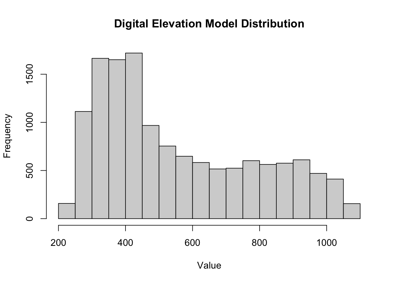

terra::boxplot(dem,
               main = "Digital Elevation Model Distribution",
               ylab = "Value")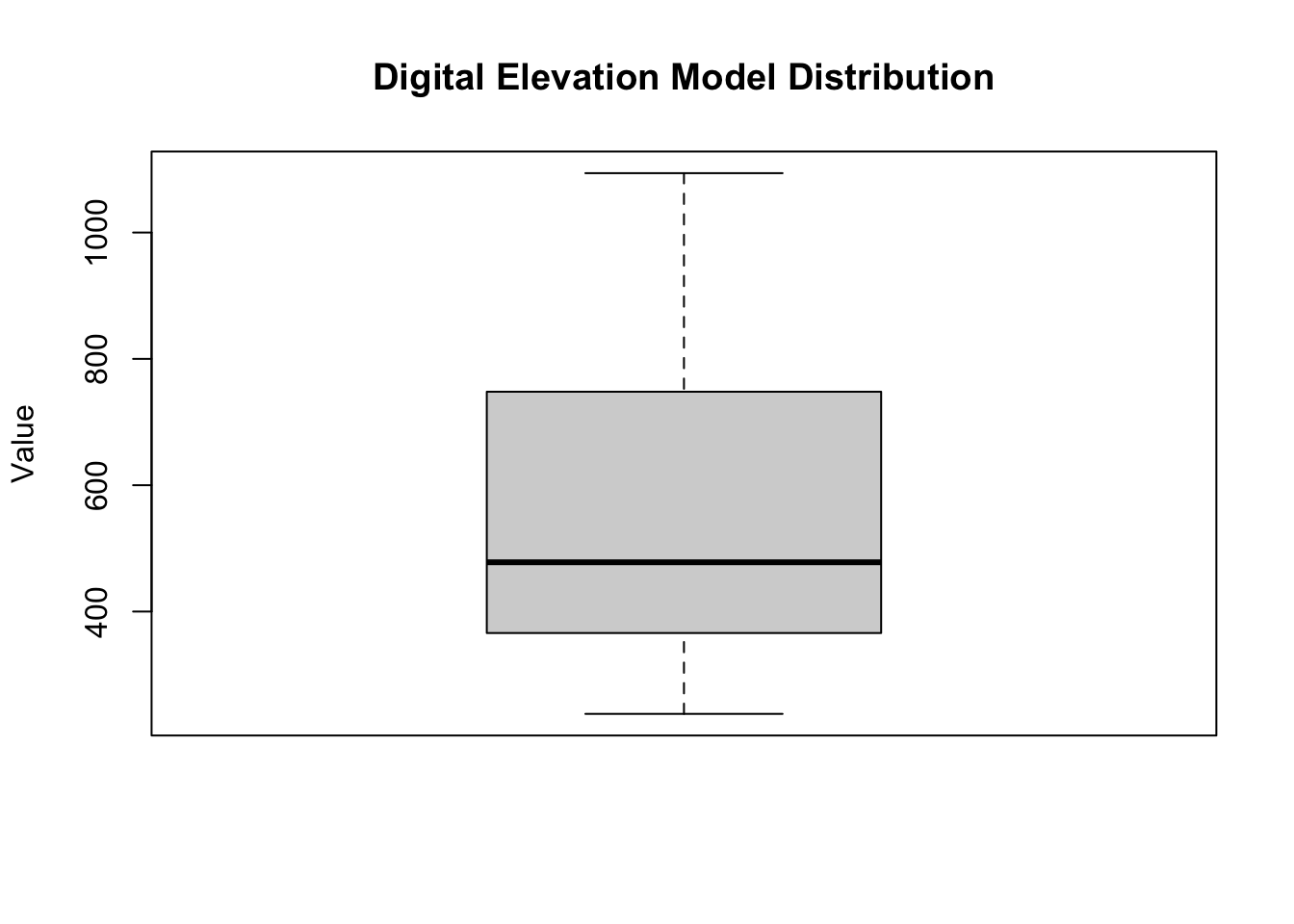

Solution

# Define a reclassification matrix
rcl <- matrix(c(-Inf, 300, 0, # values -Inf to 300 = 0
                300, 500, 1,  # values 300 to 500 = 1
                500, Inf, 2), # values 500 to Inf = 2
              ncol = 3, byrow = TRUE)

# Apply the matrix to reclassify the raster, making all cells 0 or 1 or 2
dem_rcl <- terra::classify(dem, rcl = rcl)

# Assign labels to the numerical categories

# Old version: works with newer terra, but older versions (e.g., 1.7) error with
# "[set.cats] the first column of 'value' must be numeric" because they don't accept a tibble
# levels(dem_rcl) <- tibble::tibble(id = 0:2,
#                                   cats = c("low", "medium", "high"))

# New version: a plain data.frame works with both older and newer terra
levels(dem_rcl) <- data.frame(id = 0:2,
                              cats = c("low", "medium", "high"))

# Calculate mean elevation for each category using original DEM values
elevation_mean <- terra::zonal(dem, dem_rcl, fun = "mean")
elevation_mean

    cats      dem
1    low 274.3910
2 medium 392.0486
3   high 765.2197

3. Explore NDVI and NDWI at Zion National Park

Hint: Explore the terra package to find a function that can help find the correlation!

Solution

scale_factor <- 0.0000275
offset <- 0.2

scale_function <- function(x) {
  x * scale_factor + offset
}

landsat_scaled <- terra::app(landsat, fun = scale_function)

Solution

ndwi_fun <- function(green, nir){
    (green - nir)/(green + nir)
}

ndvi_fun <- function(nir, red){
  (nir - red)/(nir + red)
}

Solution

ndwi_rast <- terra::lapp(landsat_scaled[[c(2, 4)]],
                         fun = ndwi_fun)

ndvi_rast <- terra::lapp(landsat_scaled[[c(4, 3)]],
                         fun = ndvi_fun)

plot(ndwi_rast,
     main = "Zion National Park NDWI")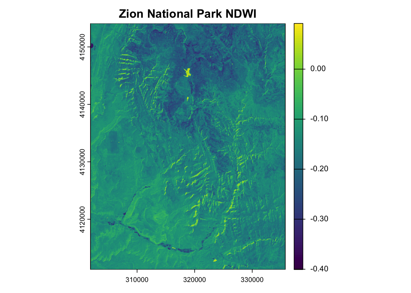

library(terra)

combine <- c(ndvi_rast, ndwi_rast) # Stack rasters

plot(combine, main = c("NDVI", "NDWI")) # Plot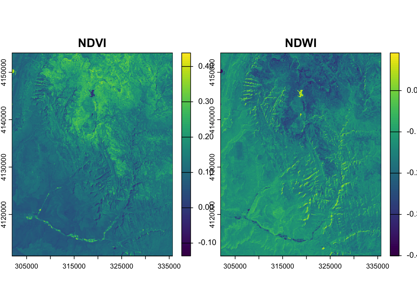

# Calculate correlation between raster layers
terra::layerCor(combine, fun = cor)

           [,1]       [,2]
[1,]  1.0000000 -0.9062336
[2,] -0.9062336  1.0000000

4. Change resolution of elevation at Zion National Park

Solution

plot(srtm)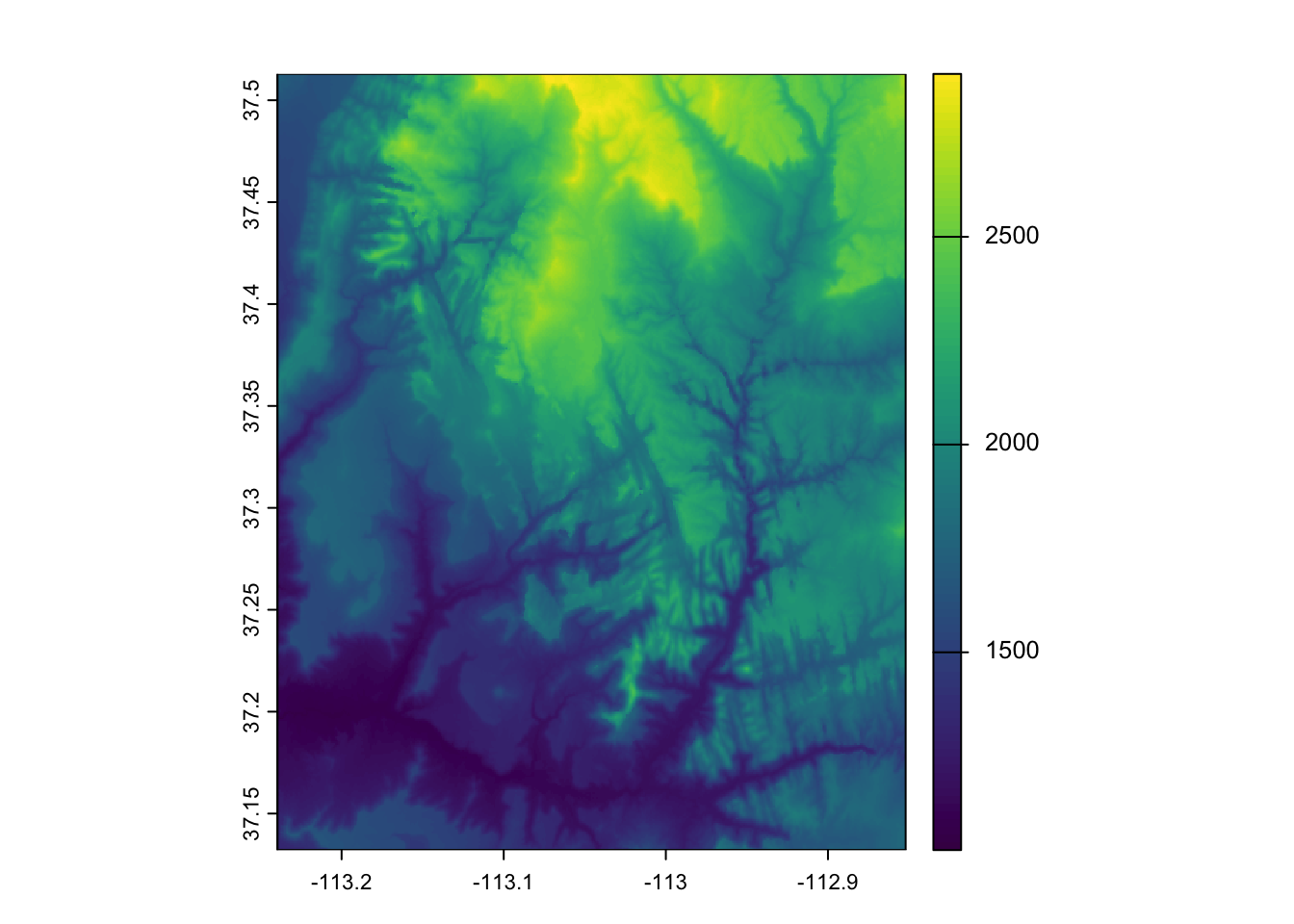

rast_template <- terra::rast(terra::ext(srtm), res = 0.01) # Create empty template

srtm_resampl1 <- terra::resample(srtm, y = rast_template, method = "bilinear")
srtm_resampl2 <- terra::resample(srtm, y = rast_template, method = "near")
srtm_resampl3 <- terra::resample(srtm, y = rast_template, method = "cubic")
srtm_resampl4 <- terra::resample(srtm, y = rast_template, method = "cubicspline")
srtm_resampl5 <- terra::resample(srtm, y = rast_template, method = "lanczos")

srtm_resampl_all <- c(srtm_resampl1, srtm_resampl2, srtm_resampl3, srtm_resampl4, srtm_resampl5)
labs <- c("Bilinear", "Near", "Cubic", "Cubic Spline", "Lanczos")

plot(srtm_resampl_all, main = labs)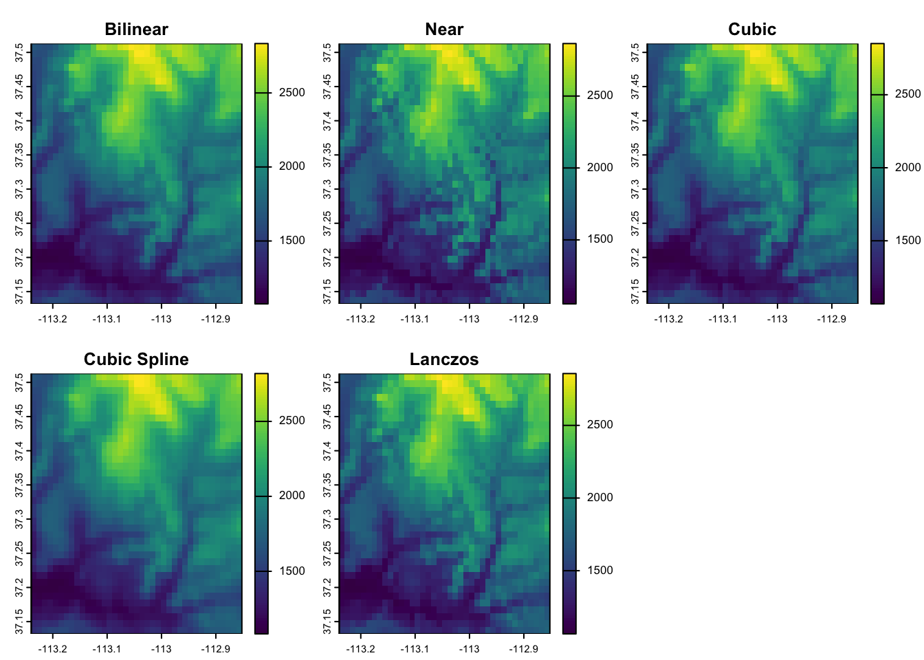

Part 2: `sf` + `stars`

1. Load the data

dem <- stars::read_stars(system.file("raster/dem.tif", package = "spDataLarge"))
landsat <- stars::read_stars(system.file("raster/landsat.tif", package = "spDataLarge"))
srtm <- stars::read_stars(system.file("raster/srtm.tif", package = "spDataLarge"))

class(srtm)   # should be "stars" in Part 2

[1] "stars"

# A stars object is a list of arrays (attributes) plus a set of dimensions
dem

stars object with 2 dimensions and 1 attribute
attribute(s):
         Min. 1st Qu. Median     Mean 3rd Qu. Max.
dem.tif   238     366    478 555.9741     748 1094
dimension(s):
  from  to  offset  delta                refsys point x/y
x    1 117  794599  30.85 WGS 84 / UTM zone 17S FALSE [x]
y    1 117 8935384 -30.85 WGS 84 / UTM zone 17S FALSE [y]

landsat # Note the third dimension, "band"

stars object with 3 dimensions and 1 attribute
attribute(s), summary of first 1e+05 cells:
             Min. 1st Qu. Median     Mean 3rd Qu.  Max.
landsat.tif  7701    8412   8739 8941.313    9258 14072
dimension(s):
     from   to  offset delta                refsys point x/y
x       1 1128  301905    30 WGS 84 / UTM zone 12N FALSE [x]
y       1 1428 4154085   -30 WGS 84 / UTM zone 12N FALSE [y]
band    1    4      NA    NA                    NA    NA

2. Explore elevation at Mt. Mongón, Perú

Solution

# Extract the array of values from the first (and only) attribute
dem_values <- as.vector(dem[[1]])

hist(dem_values,
     main = "Digital Elevation Model Distribution",
     xlab = "Value")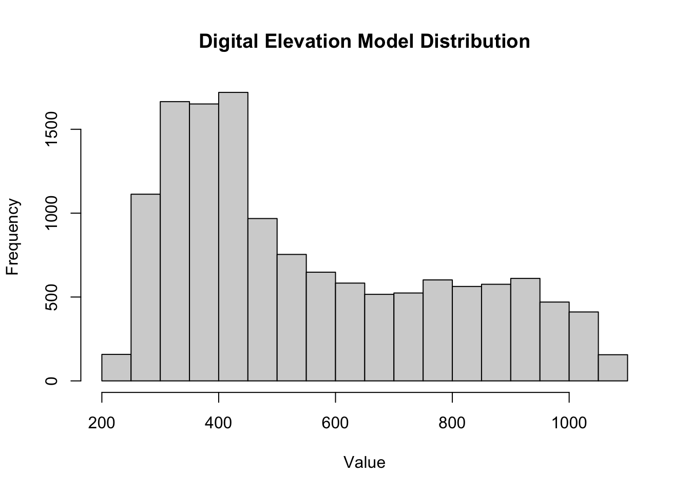

boxplot(dem_values,
        main = "Digital Elevation Model Distribution",
        ylab = "Value")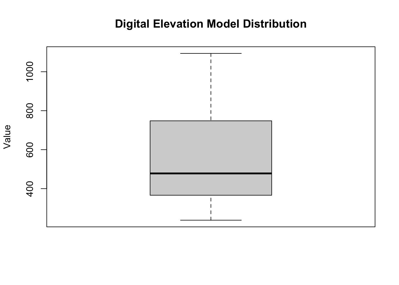

Solution

# Reclassify by cutting values into intervals, returning a factor raster
dem_rcl <- cut(dem,
               breaks = c(-Inf, 300, 500, Inf), # -Inf to 300, 300 to 500, 500 to Inf
               labels = c("low", "medium", "high"))

plot(dem_rcl, main = "Reclassified elevation")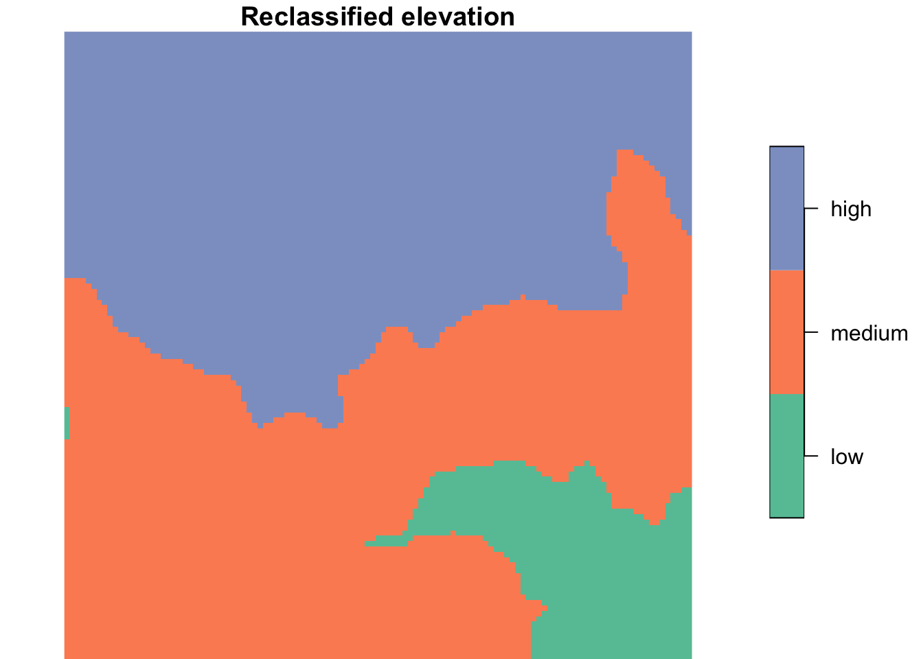

# Calculate mean elevation for each category using original DEM values
elevation_mean <- tibble(elevation = as.vector(dem[[1]]),
                         cats = factor(as.vector(dem_rcl[[1]]), levels = levels(dem_rcl[[1]]))) %>%
  group_by(cats) %>%
  summarise(mean_elevation = mean(elevation, na.rm = TRUE))
elevation_mean

# A tibble: 3 × 2
  cats   mean_elevation
  <fct>           <dbl>
1 low              274.
2 medium           392.
3 high             765.

Alternatively, we can use sf to turn the classes into polygons and then aggregate the original raster over those polygons:

# Polygonize the reclassified raster, merging cells of the same class
dem_polys <- sf::st_as_sf(dem_rcl, merge = TRUE) %>%
  group_by(dem.tif) %>%
  summarise() # Dissolve into one (multi)polygon per class

# Compute the mean of DEM values falling inside each polygon
aggregate(dem, by = dem_polys, FUN = mean) %>%
  sf::st_as_sf() %>%
  mutate(cats = dem_polys$dem.tif)

Simple feature collection with 3 features and 2 fields
Geometry type: GEOMETRY
Dimension:     XY
Bounding box:  xmin: 794599.1 ymin: 8931775 xmax: 798208.6 ymax: 8935384
Projected CRS: WGS 84 / UTM zone 17S
   dem.tif                       geometry   cats
1 274.3910 MULTIPOLYGON (((797252.2 89...    low
2 392.0486 POLYGON ((797776.7 8934706,... medium
3 765.2197 POLYGON ((794599.1 8935384,...   high

3. Explore NDVI and NDWI at Zion National Park

Hint: A stars attribute is just an R array, so base R functions work on it!

Solution

scale_factor <- 0.0000275
offset <- 0.2

# Arithmetic on a stars object is applied to every grid cell
landsat_scaled <- landsat * scale_factor + offset

Solution

ndwi_fun <- function(green, nir){
    (green - nir)/(green + nir)
}

ndvi_fun <- function(nir, red){
  (nir - red)/(nir + red)
}

Solution

# Split the "band" dimension into attributes (X1 = blue, X2 = green, X3 = red, X4 = NIR)
landsat_bands <- split(landsat_scaled, "band")
landsat_bands

stars object with 2 dimensions and 4 attributes
attribute(s), summary of first 1e+05 cells:
         Min.  1st Qu.    Median      Mean   3rd Qu.      Max.
X1  0.4117775 0.431330 0.4403225 0.4458861 0.4545950 0.5869800
X2  0.3808675 0.424235 0.4372150 0.4434250 0.4559700 0.6300725
X3  0.3624975 0.408395 0.4303675 0.4419199 0.4632575 0.7378725
X4  0.3555675 0.618495 0.6523750 0.6498339 0.6853750 0.9389525
dimension(s):
  from   to  offset delta                refsys point x/y
x    1 1128  301905    30 WGS 84 / UTM zone 12N FALSE [x]
y    1 1428 4154085   -30 WGS 84 / UTM zone 12N FALSE [y]

ndwi_rast <- landsat_bands %>%
  transmute(ndwi = ndwi_fun(green = X2, nir = X4))

ndvi_rast <- landsat_bands %>%
  transmute(ndvi = ndvi_fun(nir = X4, red = X3))

plot(ndwi_rast,
     main = "Zion National Park NDWI")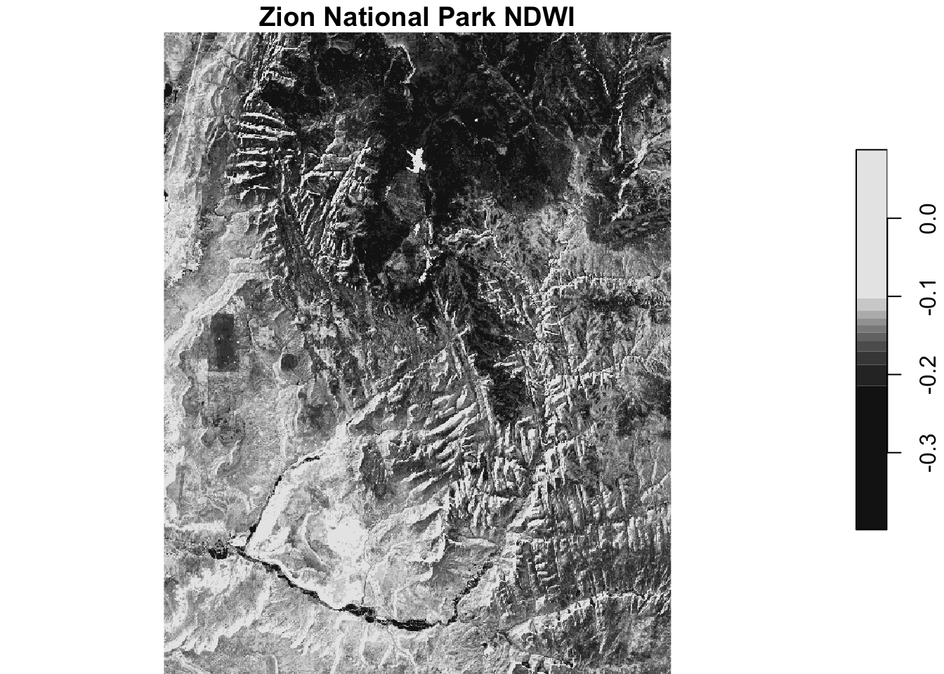

plot(ndvi_rast,
     main = "Zion National Park NDVI")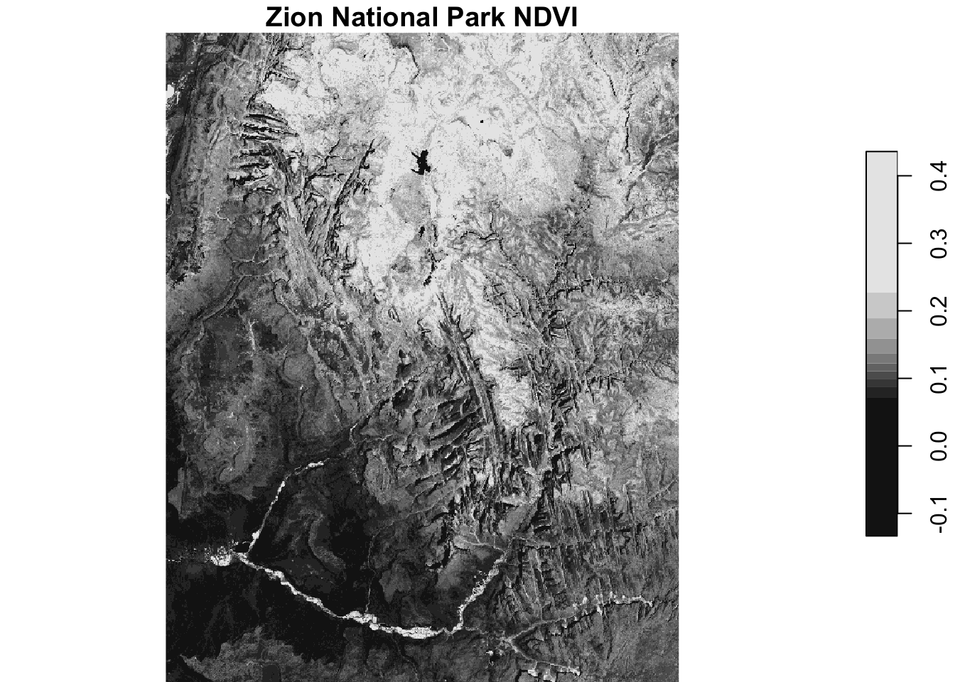

combine <- c(ndvi_rast, ndwi_rast) # Combine as two attributes

plot(merge(combine)) # Merge attributes into a dimension to plot side by side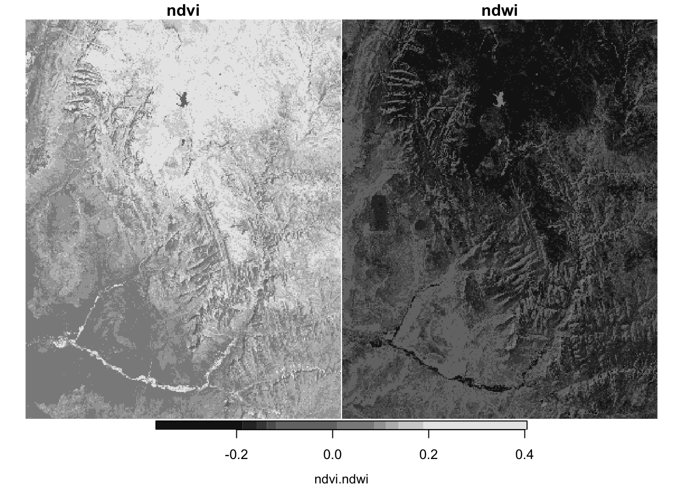

# Calculate correlation between the two attributes
cor(as.vector(combine$ndvi), as.vector(combine$ndwi), use = "complete.obs")

[1] -0.9062336

4. Change resolution of elevation at Zion National Park

Solution

plot(srtm)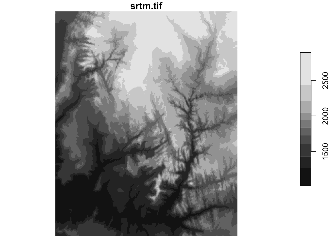

# Create empty template from the bounding box of srtm
rast_template <- stars::st_as_stars(sf::st_bbox(srtm), dx = 0.01, dy = 0.01)

# use_gdal = TRUE is needed for methods other than nearest neighbor
srtm_resampl1 <- stars::st_warp(srtm, dest = rast_template, method = "bilinear", use_gdal = TRUE, no_data_value = -9999)
srtm_resampl2 <- stars::st_warp(srtm, dest = rast_template, method = "near", use_gdal = TRUE, no_data_value = -9999)
srtm_resampl3 <- stars::st_warp(srtm, dest = rast_template, method = "cubic", use_gdal = TRUE, no_data_value = -9999)
srtm_resampl4 <- stars::st_warp(srtm, dest = rast_template, method = "cubicspline", use_gdal = TRUE, no_data_value = -9999)
srtm_resampl5 <- stars::st_warp(srtm, dest = rast_template, method = "lanczos", use_gdal = TRUE, no_data_value = -9999)

srtm_resampl_all <- c(srtm_resampl1, srtm_resampl2, srtm_resampl3, srtm_resampl4, srtm_resampl5)
names(srtm_resampl_all) <- c("Bilinear", "Near", "Cubic", "Cubic Spline", "Lanczos")

plot(merge(srtm_resampl_all))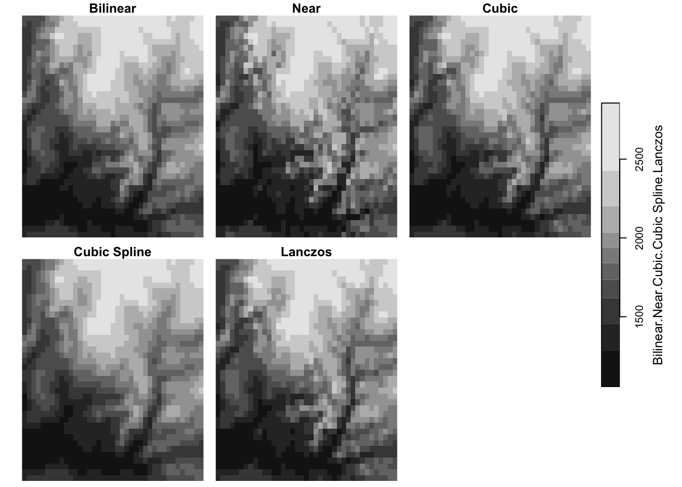

`terra` vs. `stars`: what’s the difference?

Source

The written comparison below is based on Chapter 7: Introduction to sf and stars in Spatial Data Science: With Applications in R by Edzer Pebesma and Roger Bivand.

Both packages gave the same answers above (identical class means and an NDVI–NDWI correlation of about -0.91). The difference is in how each package represents raster data.

terra (successor of raster)

raster, and now its successor terra, has long been the main R package for powerful, flexible, and scalable raster analysis.
Its data model is a 2D regular raster, or a set (stack) of raster layers. This fits a static “GIS view” of the world, where each theme is a layer.
For data that change over time, a layer stack means the user has to keep track of which layer represents what (e.g., which layer is which date or band).

stars (spatiotemporal arrays)

stars was written to support raster and vector data cubes. Raster layers, raster stacks, and feature time series are special cases of a data cube.
A stars object is a list of arrays (attributes) plus a table of dimensions (x, y, band, time, …) with fields like offset, delta, and refsys. Time is just another dimension, so time-varying raster stacks are represented directly.
It handles regular grids as well as rotated, sheared, rectilinear, and curvilinear rasters, and arrays whose spatial dimension is a set of geometries (vector data cubes).
It is tightly integrated with sf: functions share the st_ prefix, rasters can be cropped or aggregated with sf objects, and st_as_sf() converts back to sf.
It follows tidyverse design: filter(), slice(), mutate(), and transmute() work on data cubes.
It aims to scale beyond local disk size; stars_proxy objects are essentially pointers to files that are only read when needed.

	`terra`	`stars`
Data model	2D regular raster or a stack of layers	N-dimensional arrays (data cubes) with attributes and dimensions
Time-varying data	User keeps track of which layer is which	Time is a dimension of the cube
Grid types	Regular rasters	Regular, rotated, sheared, rectilinear, curvilinear, and vector data cubes
Scale	Handles data up to the size of local storage	Aims beyond local disk size using `stars_proxy` objects

How this showed up in this lab

Task	`terra` (Part 1)	`stars` (Part 2)
Multi-band data	Each band is a layer: `landsat_scaled[[c(4, 3)]]`	Bands are a dimension; `split()` turns them into attributes (`X1`–`X4`) and `merge()` reverses it
Cell-wise math	`app()`, `lapp()`	Arithmetic is passed on to the arrays: `landsat * scale_factor + offset`, `transmute()`
Reclassify and zonal statistics	`classify()` + `zonal()`	`cut()`, then `st_as_sf()` + `aggregate()` with polygons
Resampling	`resample()` to a template	`st_warp()` to a target grid; the book recommends giving the target grid as a `stars` object, as we did with `rast_template`

Get Started

Exercises

Part 1: terra

1. Load the data

2. Explore elevation at Mt. Mongón, Perú

3. Explore NDVI and NDWI at Zion National Park

4. Change resolution of elevation at Zion National Park

Part 2: sf + stars

1. Load the data

2. Explore elevation at Mt. Mongón, Perú

3. Explore NDVI and NDWI at Zion National Park

4. Change resolution of elevation at Zion National Park

terra vs. stars: what’s the difference?

Part 1: `terra`

Part 2: `sf` + `stars`

`terra` vs. `stars`: what’s the difference?