Week 3: Discussion Section

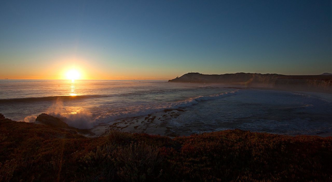
Jack and Laura Dangermond Preserve near Lompoc, CA

In this section, we’ll explore key vector operations inside the sf package using data from California. California is considered a key global biodiversity hotspot. It is home to an exceptional variety of species and ecosystems as well as high endemism. Its mix of elevation, from the highest to the lowest points in the continental U.S., and its location, near both the ocean and mountains, make it geodiverse and so biologically special. As a result, California has one of the most extensive and advanced systems of protected areas in the U.S. It currently conserves more than 25% of its land. At large, area-based conservation is complex and implementation of conservation sites has been a way for governments to displace Indigenous peoples and local communities.

Learning Objectives

Explore topological relationships with sf functions
Explore distance relationships with sf functions
Learn about spatial and distance-based joins
Practice writing error/warning messages and unit tests to diagnose outputs

1. Get Started

Create a version-controlled R Project
Add (at least) a subfolder to your R project: data
Create a Quarto document

Let’s load all necessary packages:

library(here)
library(tidyverse)
library(sf)
library(tmap)

You will be working with the following datasets:

Santa Barbara County’s City Boundaries (Santa Barbara County)
California Protected Areas Database (CPAD)
iNaturalist Research-grade Observations, 2020-2024 (via rinat)

Next, let’s download our data. Unzip and move this to your version-controlled R Project’s data folder.

sb_protected_areas <- st_read(here("data", "cpad_super_units_sb.shp")) |>  
  st_transform("ESRI:102009")

sb_city_boundaries <- st_read(here("data", "sb_city_boundaries_2003.shp")) |> 
  st_transform("ESRI:102009")

sb_county_boundary <- st_read(here("data", "sb_county_boundary_2020.shp")) |> 
  st_transform("ESRI:102009")

aves <- st_read(here("data", "aves_observations_2020_2024.shp")) |> 
  st_transform("ESRI:102009")

2. Find bird observations within PAs in Santa Barbara County

Find how many bird observations are within protected areas in Santa Barbara County and show how your output differs with a spatial subset versus a spatial join

Solution

aves_PA_subset <- sb_protected_areas[aves, ] # Subset

nrow(aves_PA_subset) # Check number of rows

[1] 35

tm_shape(sb_county_boundary) +
  tm_fill() +
  tm_shape(sb_protected_areas) +
    tm_borders(lwd = 1, col = "#fb8500") +
    tm_fill(col = "#fb8500", alpha = 0.2) +
  tm_shape(aves_PA_subset) +
    tm_dots(col = "#023047")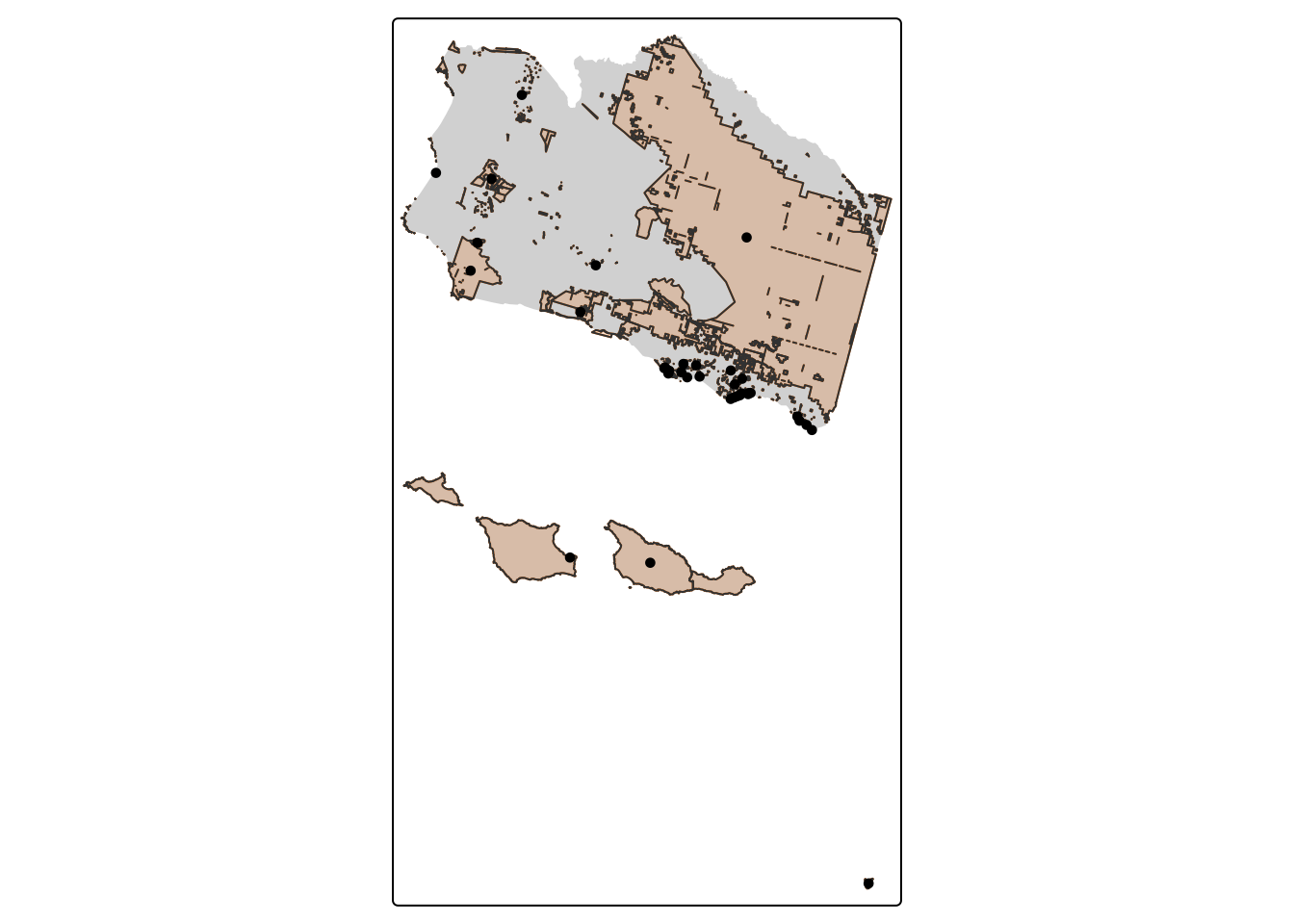

Solution

aves_PA_join <- st_join(aves, sb_protected_areas) # default: `st_intersects` 

nrow(aves_PA_join) # Check number of rows

[1] 500

tm_shape(sb_county_boundary) +
  tm_fill() +
  tm_shape(sb_protected_areas) +
    tm_borders(lwd = 1, col = "#fb8500") +
    tm_fill(col = "#fb8500", alpha = 0.2) +
  tm_shape(aves_PA_join) +
    tm_dots(col = "#023047")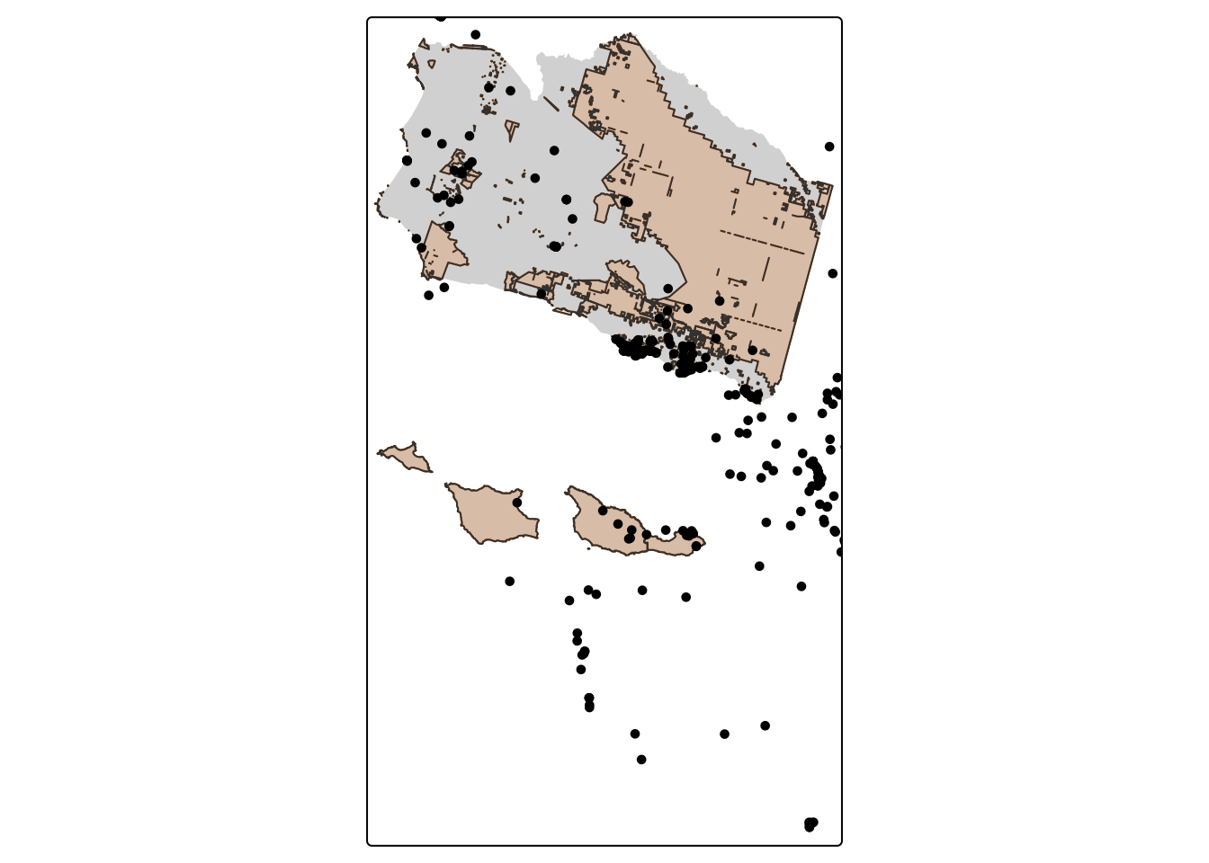

Make a 5 km buffer around the protected areas and subset buffered geometries to only those with bird observations

Solution

st_crs(sb_protected_areas)$units # Check if units are in meters

[1] "m"

PA_buffer_5km <- st_buffer(sb_protected_areas, dist = 5000) # Create 5000 m buffer around PAs

aves_buffer_subset <- PA_buffer_5km[aves, ] # Subset

nrow(aves_buffer_subset) # Check number of rows

[1] 327

tm_shape(sb_county_boundary) +
  tm_fill() +
  tm_shape(sb_protected_areas) +
    tm_borders(lwd = 1, col = "#fb8500") +
    tm_fill(col = "#fb8500", alpha = 0.2) +
  tm_shape(aves_buffer_subset) +
  tm_dots(col = "#023047")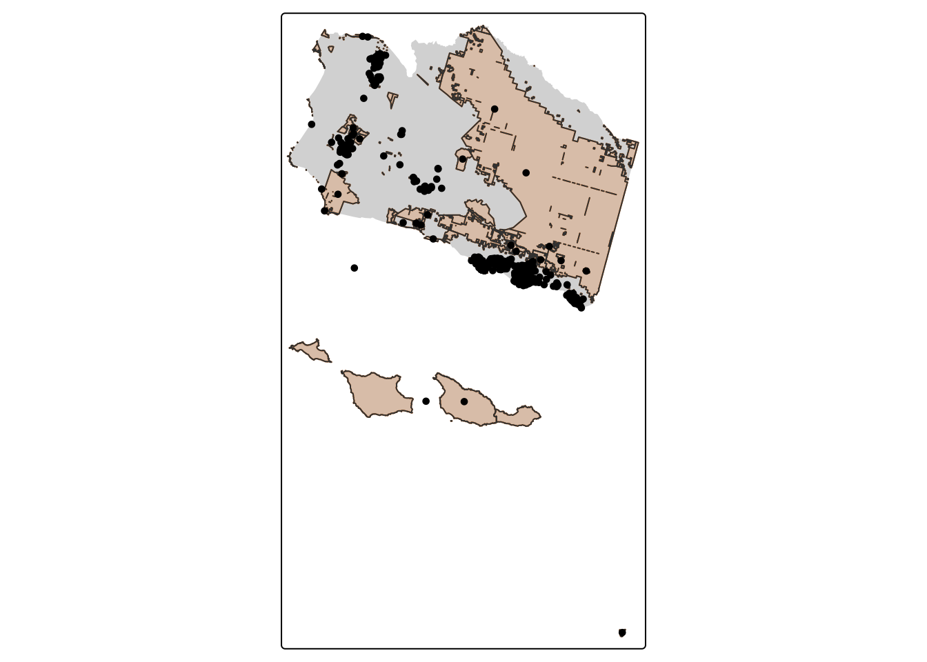

3. Find PAs within 15km of Goleta

Find the protected areas within 15 km of a city in Santa Barbara County
- Hint: Use dplyr::filter() to select a city from sb_city_boundaries

Solution

# Subset SB county to Goleta
goleta <- sb_city_boundaries |> 
  dplyr::filter(NAME == "Goleta")

st_crs(goleta)$units  # Check if units are in meters

[1] "m"

goleta_buffer_15km <- st_buffer(goleta, dist = 15000) # Create 15 km buffer around Goleta

Explore different outputs for #3 with st_intersects(), st_intersection(), and st_within()

Solution

goleta_PAs_within <- st_within(sb_protected_areas, goleta_buffer_15km)

goleta_PAs_intersect <- st_intersects(sb_protected_areas, goleta_buffer_15km)

goleta_PAs_intersection <- st_intersection(sb_protected_areas, goleta_buffer_15km)

Practice a distance-based join with st_is_within_distance()

Solution

goleta_PAs_join <- st_join(sb_protected_areas, goleta, st_is_within_distance, dist = 15000)

3. Find distance between Goleta and Dangermond Preserve

Find the distance between your city of choice and a protected area of your choice, using the geometries’ edges and the centroid

Solution

# Subset PA to Dangermond Preserve
dangermond <- sb_protected_areas |>
  dplyr::filter(UNIT_NAME == "Jack and Laura Dangermond Preserve")

danger_dist <- st_distance(goleta, dangermond) # Compute the distance between geometries edges

# Calculate the geometric center
dangermond_centroid <- st_centroid(dangermond)
goleta_centroid <- st_centroid(goleta)

danger_dist_centroid <- st_distance(goleta_centroid, dangermond_centroid) # Compute the distance between geometries edges

# Check if the distance matrices are equal
danger_dist == danger_dist_centroid

      [,1]
[1,] FALSE