Week 2: Discussion Section

Minca, Santa Marta, Magdalena, Colombia

In this section, we’ll explore key functions inside the sf package using data from Colombia. Colombia is considered one of the world’s most “megadiverse” countries, hosting close to 10% of the planet’s biodiversity. Per square kilometer, there are more bird, amphibian, butterfly, and frog species in Colombia than anywhere else on Earth. Here, ill-planned road development poses a significant threat to habitat fragmentation, wildlife movement, and water flows. The Colombian government has developed a broad set of guidelines for sustainable road development, called the Lineamientos de Infraestructura Verde Vial (LIVV) or Green Road Infrastructure Guidelines (GRI). The GRI is mandatory for all national roads across Colombia.

Learning Objectives

• Use st_read() to read multiple vector data types
• Retrieve the CRS of a vector object with st_crs()
• Transform CRS and match across all vector data types with st_transform()
• Perform dplyr attribute manipulations on sf data

1. Get Started

• Create a version-controlled R Project
• Add (at least) a subfolder to your R project: data
• Create a Quarto document

Let’s load all necessary packages:

library(tidyverse)
library(sf)
library(tmap)

You will be working with the following datasets:

• Colombia’s Terrestrial Ecosystems (The Nature Conservancy/NatureServe)
• Colombia’s Roads (Esri)
• Bird Observations (DATAVES)

Next, let’s download our data. Unzip and move this to your version-controlled R Project’s data folder.

1. Read in the data for Colombia’s ecoregions, roads, and bird observations

• Use rename() to rename the columns decimal_longitude and decimal_latitude to long and lat in the bird observation dataset
• Use st_as_sf() to convert the bird observation dataset into an sf object

Solution

col <- st_read(here::here("data", "week2-discussion", "Colombia", "Colombia.shp"))

roads <- st_read(here::here("data", "week2-discussion", "RDLINE_colombia", "RDLINE_colombia.shp"))

aves <- read_csv(here::here("data", "week2-discussion", "dataves.csv")) |> 
  as_tibble() |> 
  rename(long = decimal_longitude,
         lat = decimal_latitude) |> 
  st_as_sf(coords = c("long", "lat"), crs = 4326)

2. View class and geometry type

• Check the class() of all vector objects (including the spatially-enabled bird observation dataset)
• Use st_geometry_type() to peak at the geometry type

Solution

# View class of each object
class(col)
class(roads)
class(aves)

# View geometry type of each object
unique(st_geometry_type(col))
unique(st_geometry_type(roads))
unique(st_geometry_type(aves))

3. Select a macro ecoregion of interest

• Use filter() to select a macro region of interest from N1_MacroBi in Colombia’s ecoregions dataset
• Plot the subset using tmap

Solution

col_andean <- col |>
  # Set categorical "levels" in attribute N1_MacroBi (subregions of Colombia)
  mutate(N1_MacroBi = as.factor(N1_MacroBi)) |>
  # Subset to Andean region of Colombia
  filter(N1_MacroBi == "Andean")

tm_shape(col_andean) +
  tm_polygons() +
  tm_title("Andean Region of Colombia")

[plot mode] fit legend/component: Some legend items or map compoments do not
fit well, and are therefore rescaled.
ℹ Set the tmap option `component.autoscale = FALSE` to disable rescaling.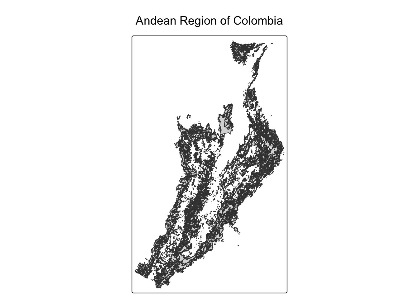

4. Play with coordinate reference system (CRS)

First, let’s use st_crs() to check the CRS and it’s units.

Solution

# View CRS of each object
st_crs(col)
st_crs(roads)
st_crs(aves)

# View units of each object CRS 
st_crs(col)$units
st_crs(roads)$units
st_crs(aves)$units

Say, you want to remove the CRS of an object, in order to “disable” its spatial features. Setting the CRS to NA with st_crs() <- NA is a brute force way to remove a CRS and “corrupt” a spatial object. Let’s do it the right way!

• Extract the longitude and latitude from the geometry column and use st_drop_geometry()

Solution

There are several ways to extract the longitude and latitude from the geometry column.

Use map() to unlist/extract

aves_df_purrr <- aves |>
  # Extract lat & long from geometry column
  mutate(lon = unlist(purrr::map(aves$geometry, 1)), # longitude = first component (x)
         lat = unlist(purrr::map(aves$geometry, 2))) |> # latitude = second component (y)
  st_drop_geometry() # Remove geometry column now that it's redundant

Use st_coordinates() to extract/assign

aves_df_st_coords <- aves %>%
  dplyr::mutate(lon = st_coordinates(.)[,1], # Assign first matrix item to "lon"
                lat = st_coordinates(.)[,2])  %>% # Assign second matrix item to "lat"
  st_drop_geometry() # Remove geometry column now that it's redundant

• Convert long and lat into a geometry again with st_as_sf() to obtain a proper sf data frame

Solution

Convert to an sf object with st_as_sf()

aves_df_purrr <- aves |>
  st_as_sf(coords = c("lon", "lat"), crs = 4326)

5. Make a map

• Check that the CRS of the ecoregions and roads datasets match
• Transform CRS of the bird observations dataset using st_transform() to match with the other datasets
• Use tmap to plot the ecoregions, roads, and bird observations together

Solution

# Boolen check if CRS match between 2 datasets
st_crs(col) == st_crs(roads)

# Transform bird observation dataset into same CRS as other Colombia dataset
aves <- st_transform(aves, crs = st_crs(col))

tm_shape(col) +
  tm_polygons() +
  tm_shape(roads) +
  tm_lines() +
  tm_shape(aves) +
  tm_dots() +
  tm_title("Colombia ecoregions, roads,\nand bird observations")