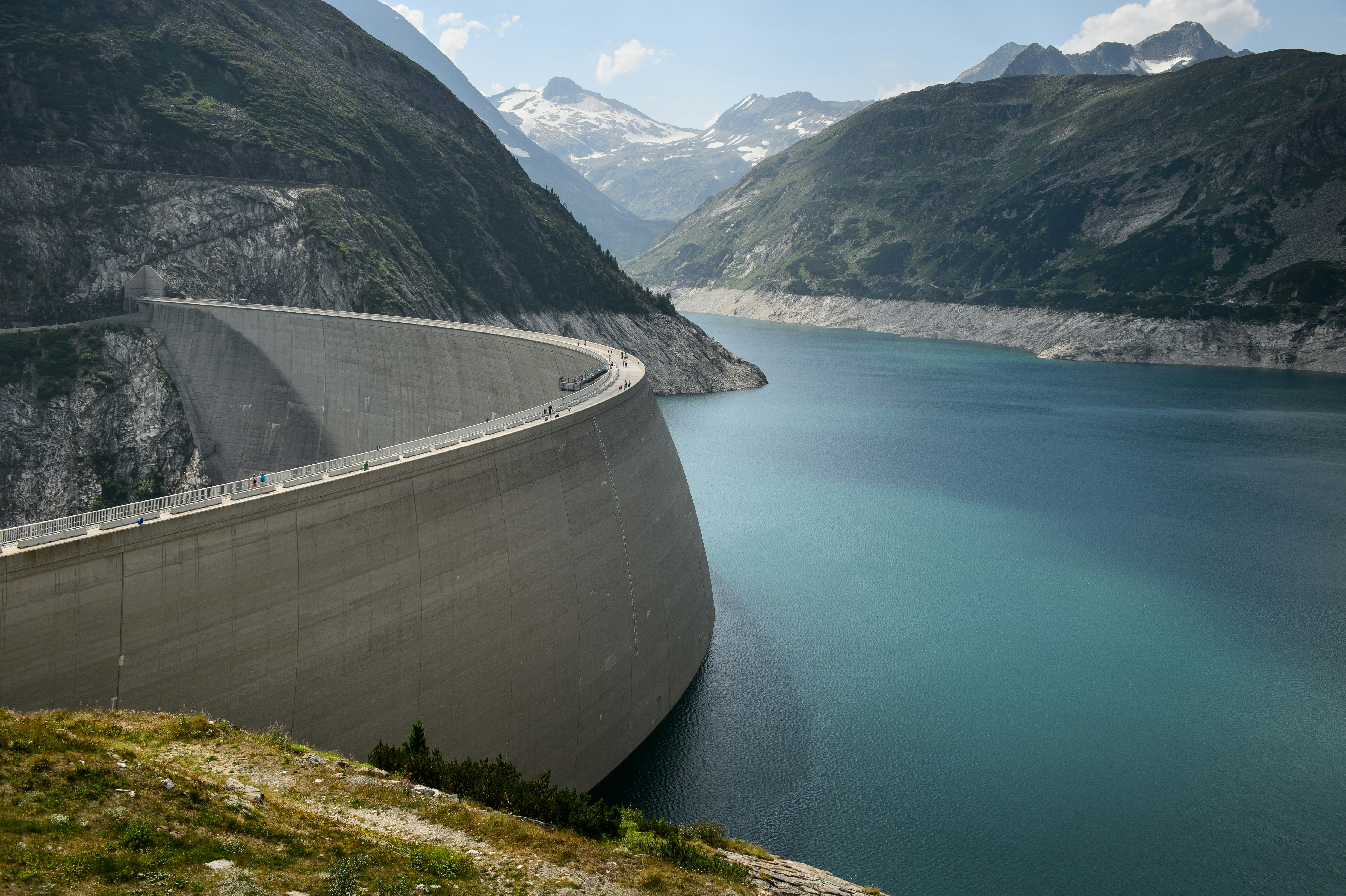
Kölnbrein Dam in Austria
In this section, we’ll refresh our data wrangling skills and refamiliarize some key functions, using a subset of the Global Dam Watch (GDW) database. This data source brings together open-access, georeferenced regional and global dam data, in order to improve our understanding of the environmental effects of dams and flood risks.
What’s up with dams?
Dams can offer many advantages as a renewable energy, but they can also pose several risks on agriculture, river connectivity, and biodiversity. On the one hand, while dams help manage water flow, they also slow it down and raise downstream water temperatures, which can encourage harmful algae and parasites. This can further drive biodiversity loss, where dams already block fish migration, fragment habitats, and trap sediment. Datasets like GDW provide increased transparency for water and biodiversity management.
1. Get Started
- Create a version-controlled R Project
- Add (at least) a subfolder to your R project:
data
Let’s install and load all necessary packages:
packages <- c("here", "janitor", "tidyverse", "sf", "terra", "tmap", "spData", "spDataLarge", "geodata", "kableExtra", "viridisLite")
installed_packages <- packages %in% rownames(installed.packages())

if (any(installed_packages == FALSE)) {
  install.packages(packages[!installed_packages])
}library(here)
library(janitor)
library(tidyverse)
library(sf)
library(kableExtra)Next, let’s download our GDW data subset to practice our data wrangling skills from EDS 221. Unzip and move this to your version-controlled R Project’s data folder.
2. Load Data
- Read in the
gdw.csvfile asgdw_df(and point to the filepath with help ofhere()) - Use the
|>or%>%operator to pipe yourread_csv()output toclean_names()
Solution
gdw_df <- read_csv(here("data", "gdw.csv")) |>
  clean_names() # Convert variable names to lower snake case
3. Data Exploration
- Show the first and last 10 rows of
gdw_dfand usekable()to make nice HTML tables - Print the number of rows and number of columns in
gdw_df - Print the column names in
gdw_df
Solution
head(gdw_df, n = 10) |>
  kable()

tail(gdw_df, n = 10) |>
kable()dim(gdw_df)
nrow(gdw_df)
ncol(gdw_df)names(gdw_df)4. Index, Summarize, Subset Data
- Use indexing brackets to extract the
gdw_dfcolumn containing country names as a vector and data frame - Use
group_by()andsummarise()to find the number of dams by dam type ingdw_df - Make a subset called
sub_damthat only contains entries fordam_type == "Dam" - Re-order
gdw_dfby ascending order of installation year
Solution
country_df <- gdw_df[, "country"]
country_vec <- gdw_df[["country"]]
gdw_df |>
group_by(dam_type) |>
summarise(count = n()) |>
ungroup()sub_dam <- gdw_df |>
filter(dam_type == "Dam")gdw_df <- gdw_df |>
arrange(year_dam)5. Data Visualization
- Make a bar graph of average height of dam/barrier in meters (
dam_hgt_m) by country - Make a scatterplot of height of dam/barrier versus representative maximum storage capacity of reservoir in million cubic meters (
cap_mcm)
Solution
gdw_df |>
  group_by(country) |>
  summarize(mean_dam_hgt_m = mean(dam_hgt_m, na.rm = TRUE)) |>
  ungroup() |>
  ggplot(aes(x = country, y = mean_dam_hgt_m)) +
    geom_bar(stat = "identity") +
    labs(x = "Country",
         y = "Average height of dam/barrier in meters") +
  theme_minimal() +
  theme(axis.text.x = element_text(angle = 45, hjust = 1, vjust = 1))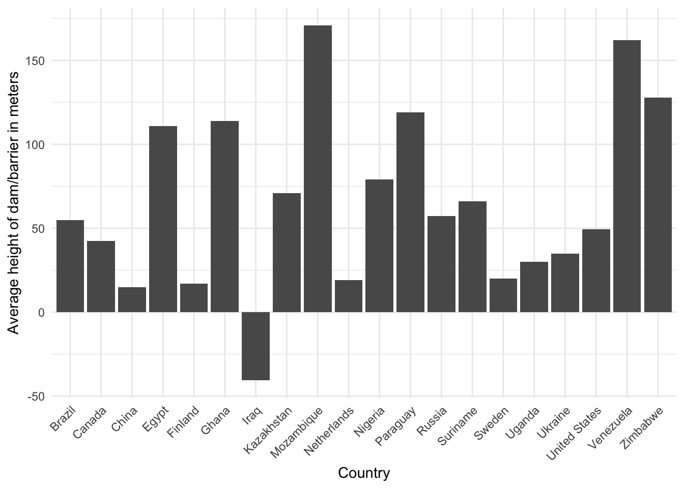
ggplot(data = gdw_df,
      aes(x = cap_mcm, y = dam_hgt_m)) +
  geom_point() +
  labs(x = "Storage capacity of reservoir in million cubic meters",
       y = "Height of dam/barrier in meters") +
  theme_minimal()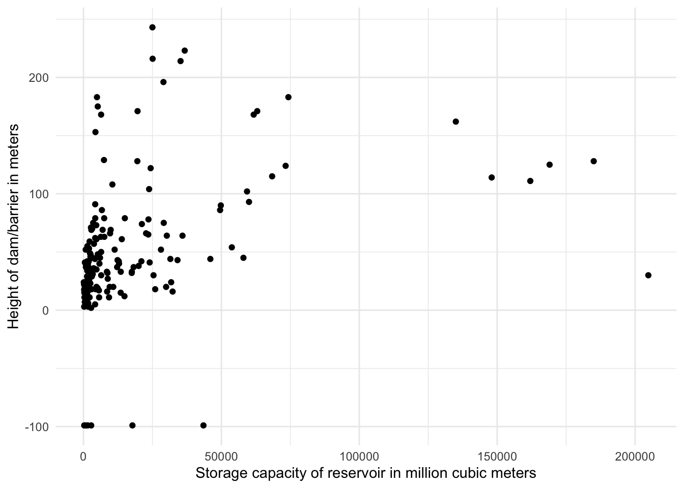
6. Looking Ahead
We have practiced wrangling a data.frame object, but gdw_df also has a shape column, which contains point coordinates (longitude and latitude). Let’s print the first 3 rows of this column and take a look at its class.
head(gdw_df$shape, n = 3)[1] "c(-97.8635419999999, 53.696359)" "c(-75.794246, 44.480557)"
[3] "c(104.321875, 52.2343930000001)"class(gdw_df$shape)[1] "character"While gdw_df contains spatial information, it needs to be spatially-enabled to be a spatial object. We use the sf package to do this. Over the next few weeks, you will be using the function st_read() (or read_sf()) to read all your shapefiles and geodatabases.
gdw_st <- st_read(here("data", "gdw.gdb")) |>
  clean_names() # Convert variable names to lower snake case
gdw_sf <- read_sf(here("data", "gdw.gdb")) |>
clean_names() # Convert variable names to lower snake case